Using Smart Load Flow in SINCAL
The Basics
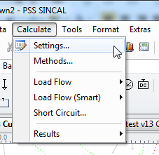
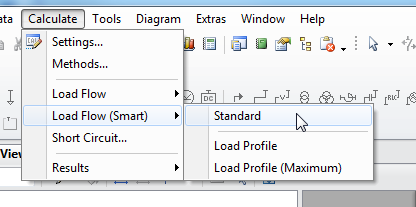
If you have the smart load module license, and the model you have opened has been converted to a smart load database using the smart load database conversion tool, the smart load flow function in SINCAL is invoked via the Calculate menu as illustrated below.

If you do not see the Load Flow (Smart) option, the model has not been converted.
Before running a Smart Load, a few settings need to be entered, as per the menu below.
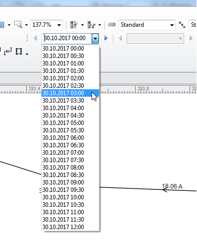
The date to use for the smart load calculation is entered into the “Basic Data” tab of the calculations settings dialogue, as illustrated below. This date would typically be a maximum demand day, and this could be found by using the Energy Workbench trend displays to find the top demand days for a feeder in the scope of the study.
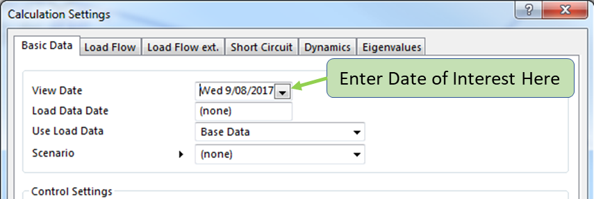
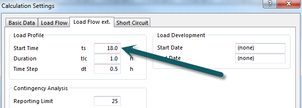
Once the day has been chosen, the time to start the study can be entered, along with the duration of the study and the time interval between each study. It is possible to run a study over more than one day.
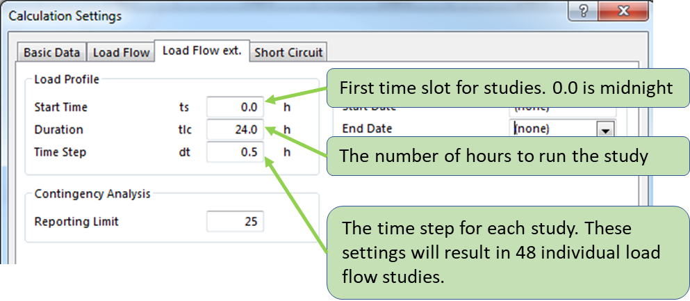
note
The AMI aggregated data used by the smart load plugin is stored as 30 minute interval data. When a time step of less than 0.5 (30 min) is picked, the smart load plugin will interpolate between the 30 minutes samples.
Settings to Avoid
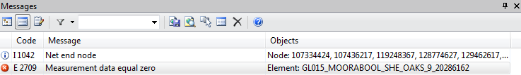
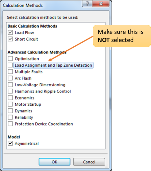
In the Calculate->Methods dialog, you need to make sure the Load Assignment and Tap Zone Detection is not selected.
If this is selected, and there are any points with missing load data, as illustrated below, the smart load function will fail.
Storing Results
The smart load flow will write a lot of data back to the SINCAL results in the MS Access database. For studies of large models over multiple days, this can result in un-acceptable performance issues – the time taken to write the data back can become excessive.
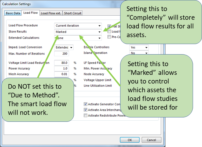
If you are only interested in a small subset of the results, you can control which parts of the network will have the results stored back to the database
danger
Do not use the “Due to Method” option. No results will be stored for smart load.
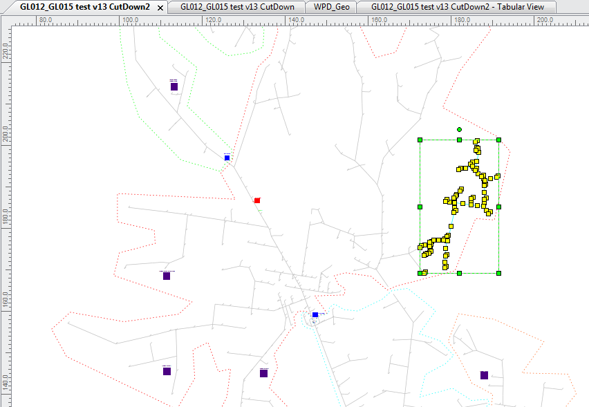
If Marked is selected, the assets that will have their results stored are selected by selecting the area of the network you want the results stored for, as illustrated below.
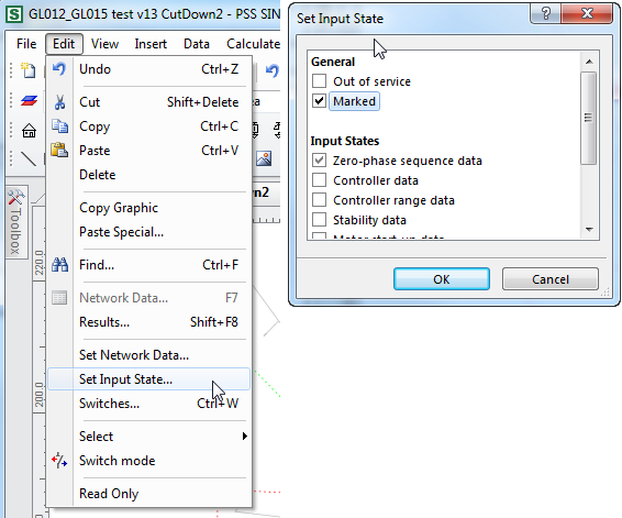
Then picking Edit->Set Input State, as illustrated below, and ticking the Marked option. Only the selected assets will have their smart load results stored. In many cases, this will not be necessary as the time interval selected and size of the network will not be so large that it is needed. However, for models with more than 500 distribution transformers, and time periods for the study of greater than one day, the performance can degrade.
Viewing the Results.
Once you have run a smart load study, you can view the results of each time slice by enabling View->Toolbars->Results. This will then let you step through each time slice.
Adding and Viewing Voltage Curves
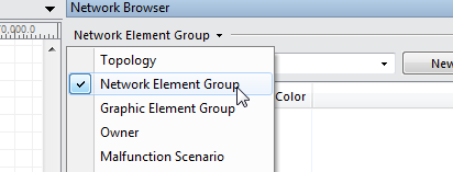
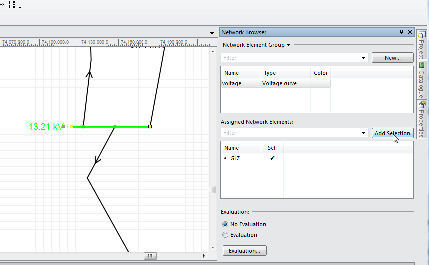
Voltage curves provide trends of voltage against distance for a load flow study. Follow the steps below to make voltage curves work with a Smart Load model. With the model loaded into the SINCAL application, under the Network Browser panel, select Network Element Group.
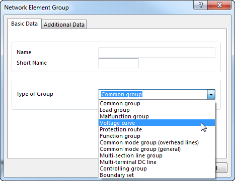
Click the New button to create a Voltage Curve Element.
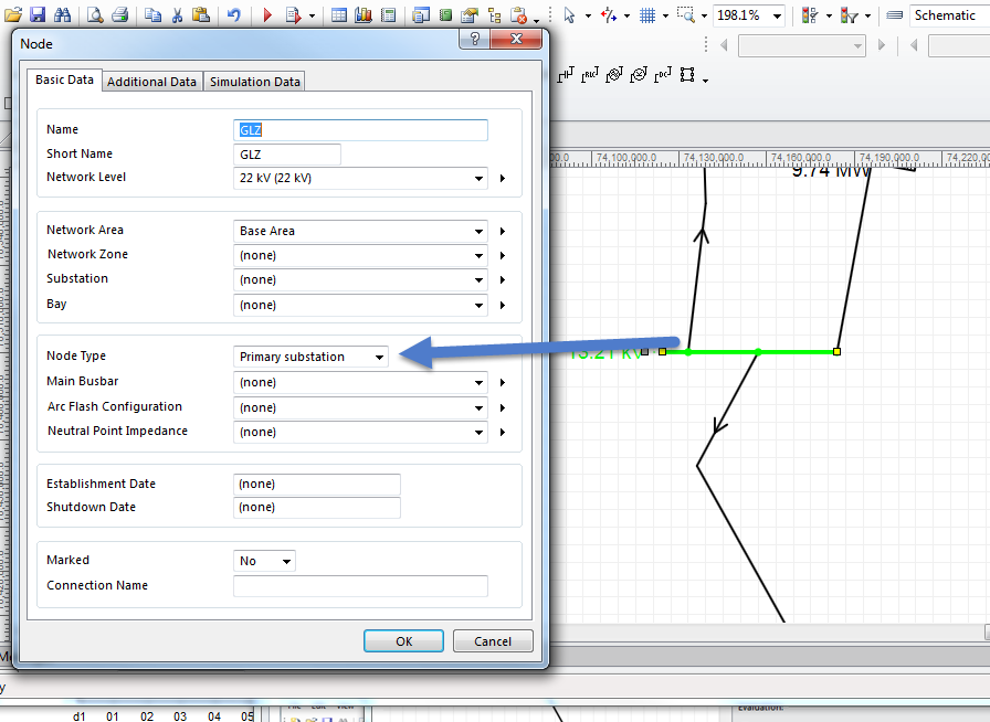
Select a primary zone substation node type, and press the Add Selection button at the bottom of the network browser panel.
Once this has been done, a load flow study using Smart Load flow can be invoked. For the results to appear in a voltage curve, the Standard option must be selected under the Load Flow (Smart) menu.
When this option is picked, the time used for the load flow study will be the Start Time in the Load Flow ext. tab. The date for the study will be in the View Date field in the Basic Data tab.
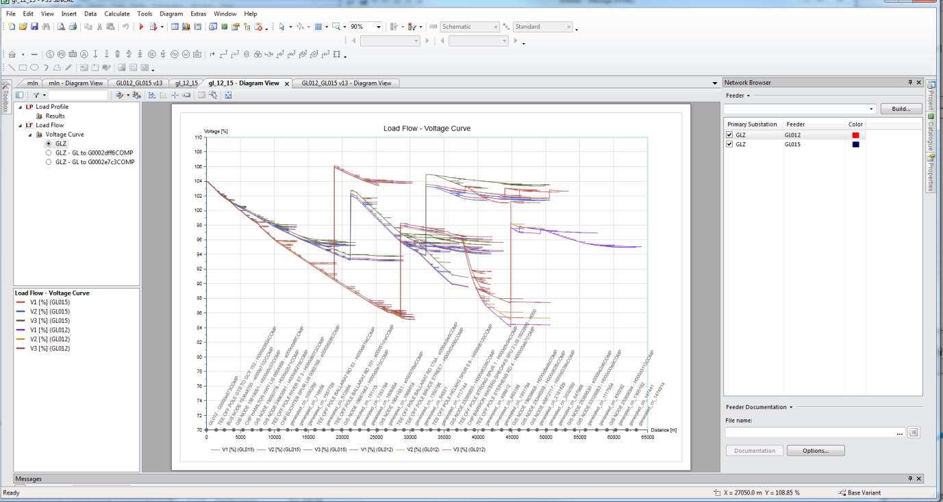
After the load flow study has executed, the Diagram View icon can be pressed in the main toolbar.
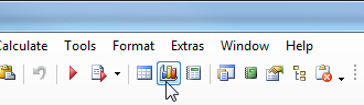
Pressing this will bring up a display showing the voltage drop for each feeder under the Load Flow group.
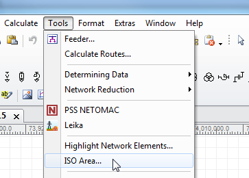
Another way to visualise voltage in the network is to use the ISO Area… function, which is invoked from the Tools menu.
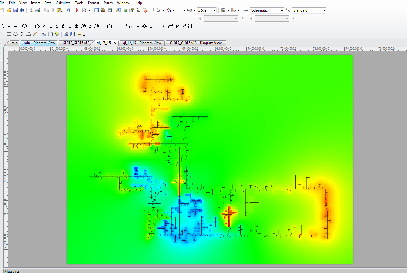
Invoking this will bring up a dialog box. Ensure the Area Definition is set to Page, and the Visualisation type is set to Vmin/Vn to see a visualisation of voltages in the network. The colour range can be adjusted by right clicking on the colour icons at the bottom of the dialog box.
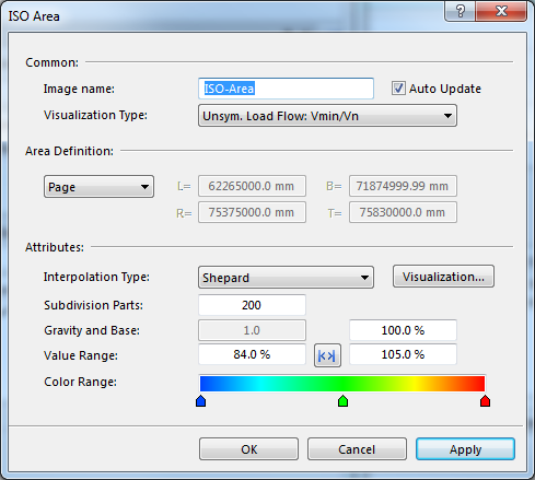
Press the Apply button to display the ISO area.
tip
ISO areas can be removed by selecting: Tools->Remove Temporary Images
Dealing With Missing Data
What happens if load data is missing, or has a 0 value, for a distribution transformer?
- If there really is no load for a time interval for that transformer, that is, the transformer is found, but it is reporting a 0 value for load, the a warning will be produced in the SINCAL message log to indicate that “Power is equal to 0”. Any other values entered into the Load element in SINCAL will be not be substituted.
- If there is a mismatch between the SINCAL database load point ID and the Energy Workbench Load point ID, or there are no load readings for the ID supplied, no warning will be given in the SINCAL message log, and the values in the Load element that would be used for a normal load flow study will be used for the load.