GIS Plugin
The Energy Workbench GIS Plugin allows detailed analysis of load at the distribution substation and LV network level. Users interact with the GIS to trace out portions of the LV network, and then add or remove supply points to create composite load trend displays of predicted maximum demand, based on historical data.
Setting Up The GIS Display
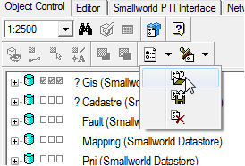
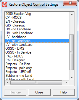
In order to user the EWB functions, the LV network needs to be made visible in the GIS display. The object control setting “LV – no Landbase” or “LV - with Landbase” are the recommended display controls to use, as illustrated.
Functions
All functions are accessed via the Tools->Tracer dialog in the GIS client. Three traces have been added to the “Trace” drop down:
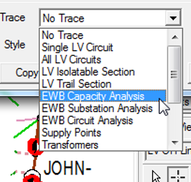
- EWB Capacity Analysis. This allows a “helicopter” view of maximum demand load profiles for a cluster of distribution transformers in close proximity to one another. The intent is to provide a quick assessment of candidates for load transfer.
- EWB Substation Analysis. This allows analysis of the impact of adding or removing multiple supply points from a distribution transformer.
- EWB Circuit Analysis. This allows analysis of the impact of adding or removing multiple supply points from individual circuits on a distribution transformer, or the load on the selected circuit.
EWB Capacity Analysis
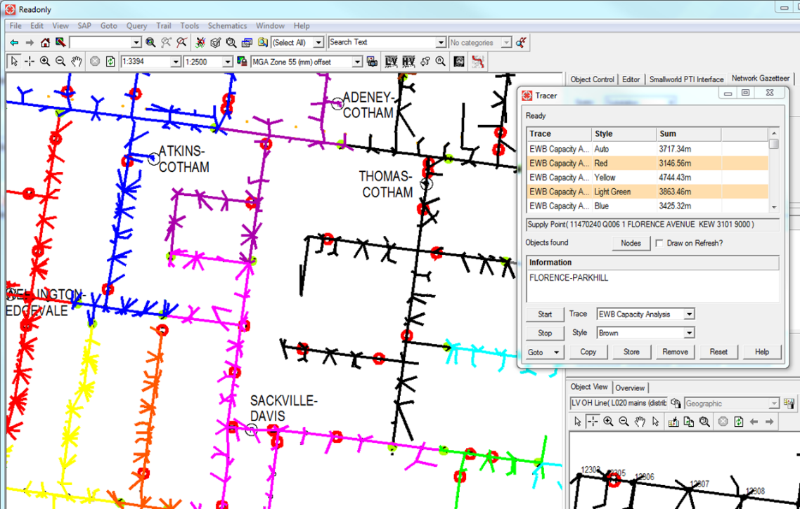
To invoke the Capacity Analysis function, an LV asset is selected, and the EWB Capacity Analysis trace executed, as illustrated in the image below.
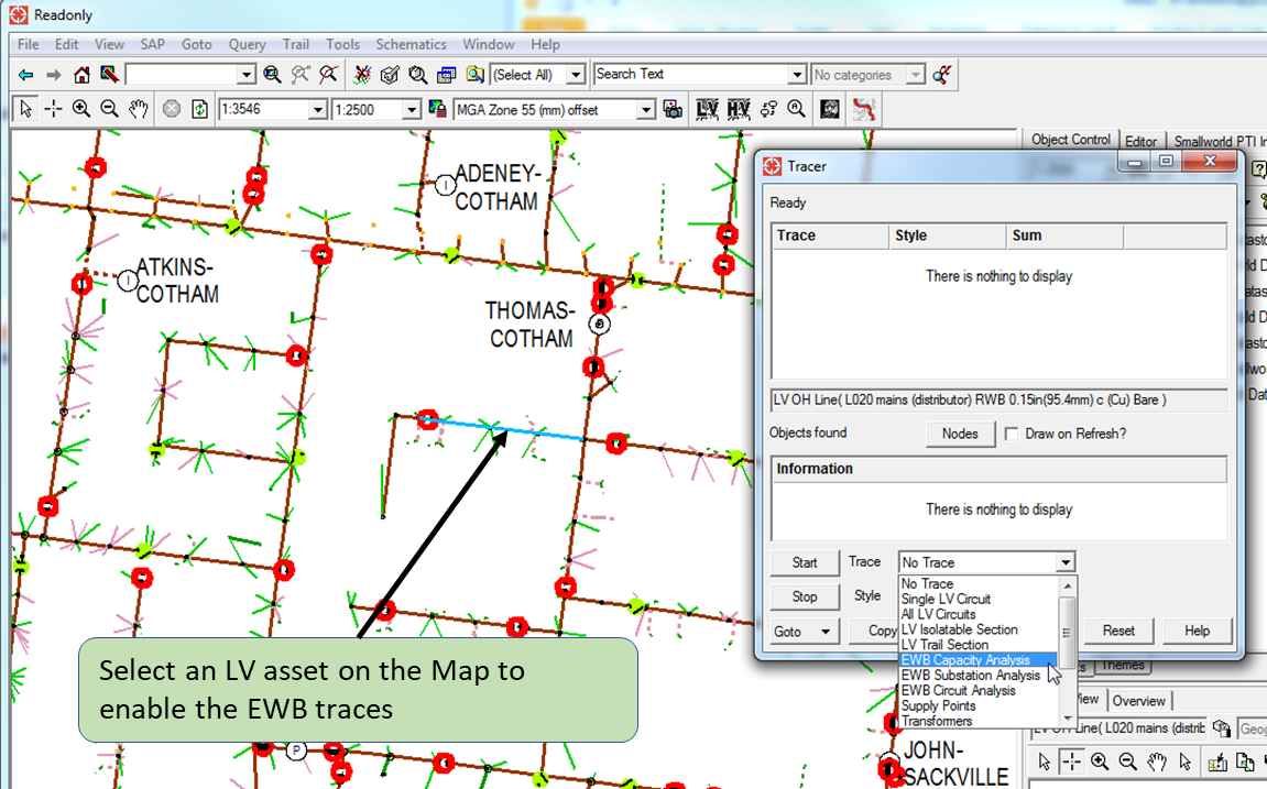
This will result in all distribution transformers than can be “reached” through open points, from the transformer connected to the selected asset being traced out, whether they are on screen or not. The GIS client should look something like the illustration below. Once the trace is finished, a browser window will be opened, and trend lines displayed for all the distribution transformers encountered in the trace, as illustrated on the following page.
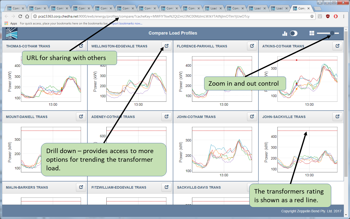
This display provides a fast, high level view of all transformer loading in the immediate vicinity of the transformer of interest, including load profile shape.
The top 5 Maximum Demand profiles for the past 2 years are displayed for each transformer.
EWB Substation Analysis
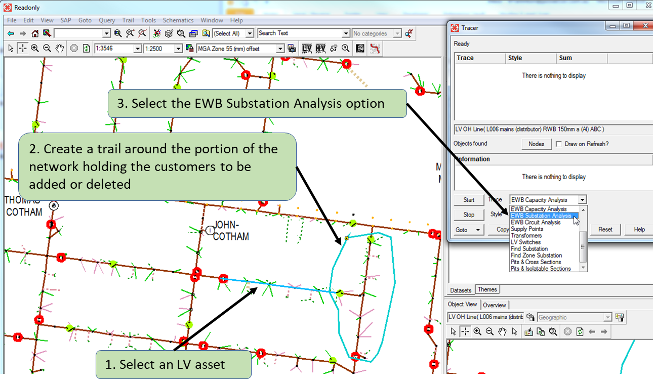
The EWB Substation Analysis function allows trend lines to be generated showing a simulation of the load profile that would be experienced by the transformer on maximum demand days if collections of specific customers were added or deleted. The steps required to use the function are illustrated below.
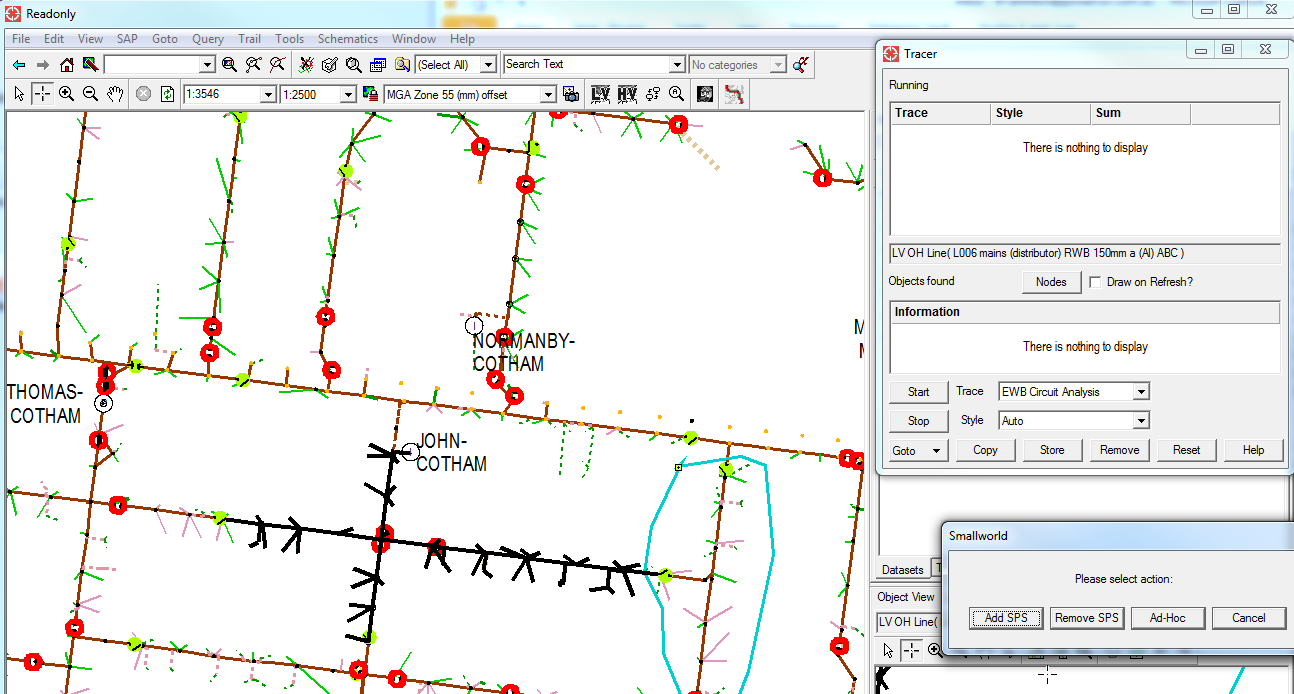
Selecting the ‘EWB Substation Analysis’ option will result in the following dialog box being displayed.
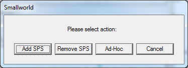
The Add SPS button will add the supply points contained within the trail for the top 5 maximum demand days for the distribution transformer to the transformers aggregated load. The Remove SPS button will remove the supply point load, and the Ad-Hoc button will summate just the load on the supply points within the trail.
Maximum Demand Algorithm
The algorithm to calculate the maximum demand works like this:
- A Trace is performed to from the selected LV asset to find its transformer. In the example above, this is the JOHN-COTHAM transformer. This can be checked by executing one of the other LV Traces in the Tracer tool prior to executing the EWB Substation Analysis trace.
- The top 5 maximum demand days for the traced transformer are then found – these days are then used to seed a maximum demand calculation for the combined load.
- The combined load is then calculated by summating the combination of supply points required for the composite load, using the most recent list of supply points, for each the transformers maximum demand days. If the “Remove SPS” option is picked, the supply points contained within the trail will be removed as supply points on the transformer. If the “Add SPS” option is picked, the supply points will be added to the supply points already on the transformer. If the “Ad-Hoc” option is picked, only the load for the supply points contained within the trail will be used to produce load trend lines for the transformers maximum demand days.
- If a supply point that is part of the calculation was not connected to the transformer on one or more of its maximum demand days, the maximum demand for the supply point since it came into existence will be used for its contribution to the calculated load profile.
The results will be displayed as a series of trend lines, as illustrated below:
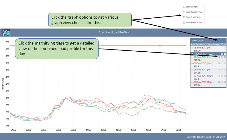
The Combined Load Profiles that would result if the selected supply points are added or removed (depending on the option chosen) for the 5 maximum demand days are drawn.
The legend on the right show the dates and day of the week for each maximum demand day. A red line is shown at the top of the screen for the transformer rating.
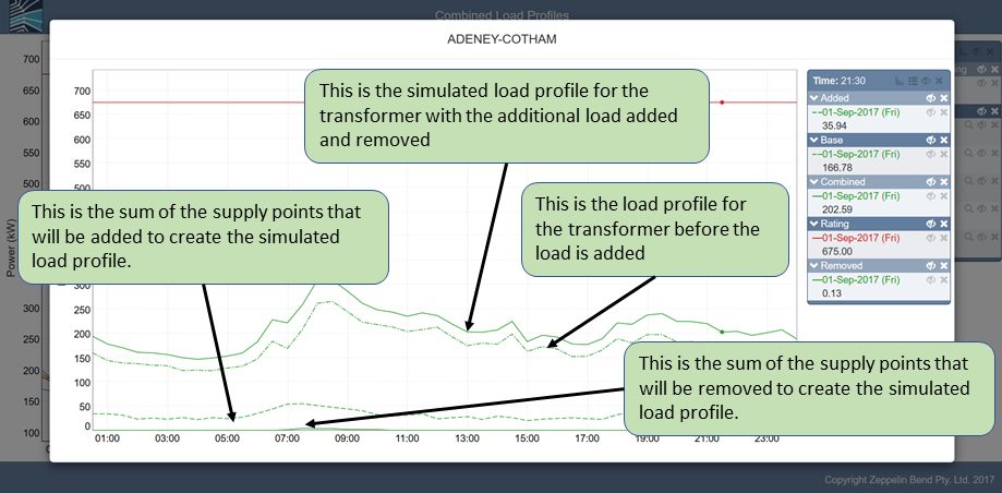
Clicking on the magnifying glass will generate a view similar to the following screen capture:
The legend on the right has buttons for graph view options and tabular view as shown below:
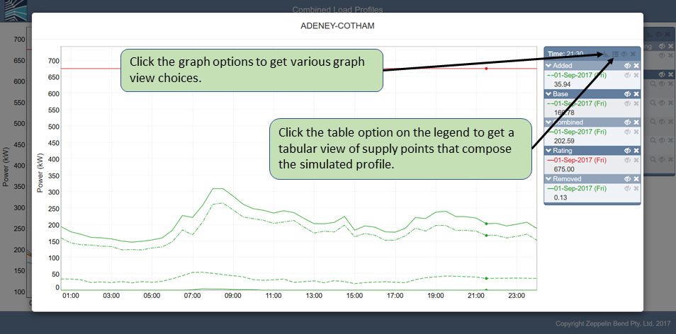
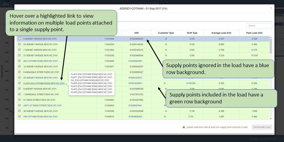
Clicking on the tabular view button brings up a tabbed view with tables that list supply points which compose the selected load profile.
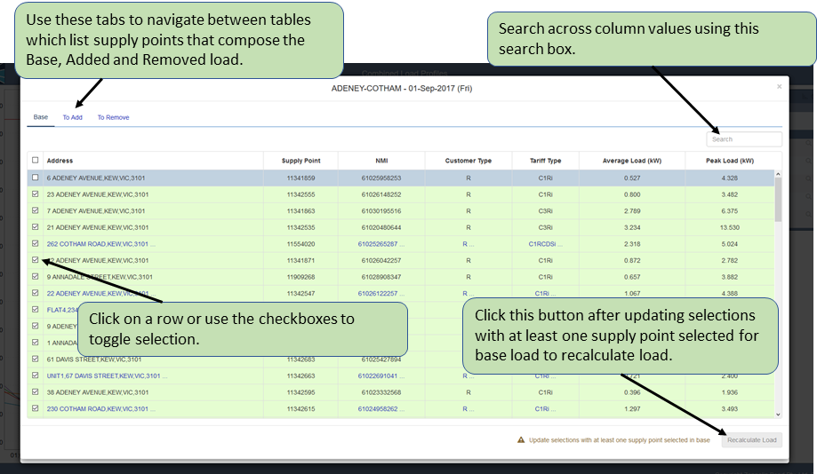
Understanding the Tabular View
- Supply points which are included in the respective load profile are preselected with a green background.
- Supply points which are not included are unselected with a blue background.
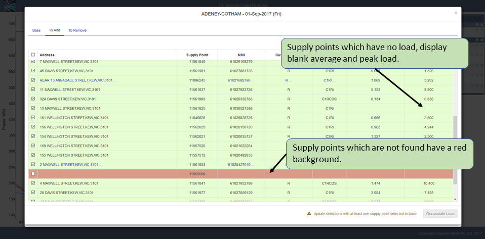
- Supply points which are not found are unselected with a red background.
- Supply points which have no attached meter information or load for the selected date have a blank for the corresponding column value.
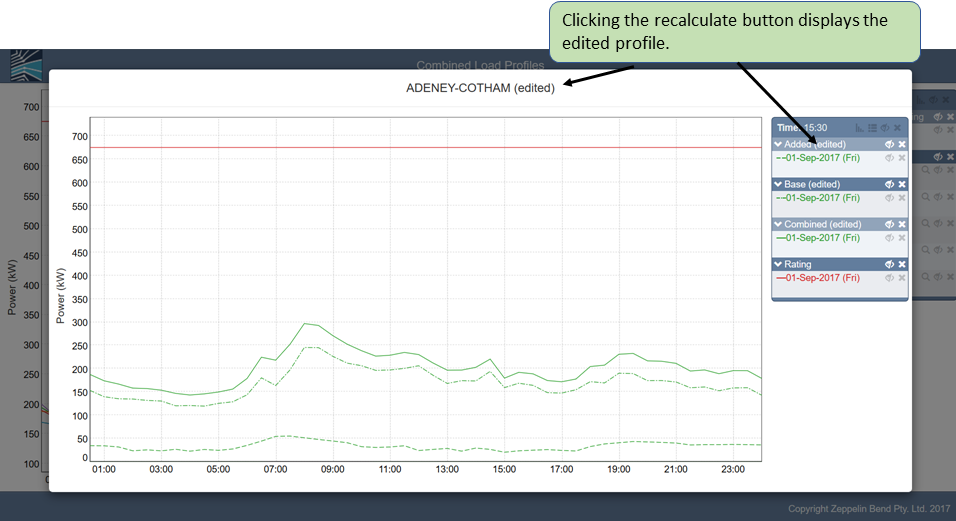
Recalculating Load
The Recalculate Load button is disabled everytime the Tabular View is opened. To enable the button, table selections must be updated and a mininum of one supply point must be selected from the Base table.
After clicking the Recalculate Button, the graph is updated with the edited simulation of the load profile.
EWB Circuit Analysis
The EWB Circuit Analysis function is similar to the EWB Substation Analysis function, except it performs the analysis on an individual circuit on the distribution transformer.
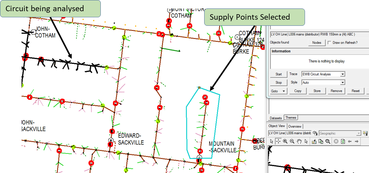
In the example above, a single circuit has been traced, a collection of supply points selected in a trail, and the EWB Circuit Analysis function picked.
This results in a set of trend lines in the same way as for the substation analysis, but with the simulated load profile consisting of the circuit load summated with the supply points.
It is possible to select supply points that are not adjacent to the circuit or transformer being analysed, for both the substation and circuit analysis functions, as illustrated below.
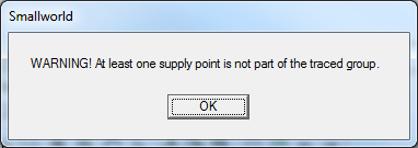
In this case, the following warning dialog will be shown if the option selected is Ad Hoc. This is purely for information purposes, the analysis will proceed anyway.
note
If no trail is selected, the EWB Circuit Analysis function will show a trend line of the top 5 MD days for the circuit.
Sharing the Results
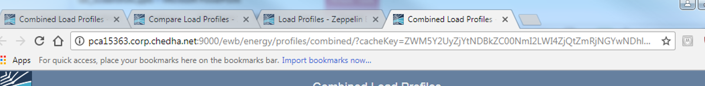
The combined load profiles may be readily shared by copying the link in the browser address bar into an email, along with images or any other material. The link will remain active for a month or more (admin configurable).
Displaying Supply Points Added or Removed
The details of the supply points and NMI’s involved in the production of the simulated load profile are copied to the clip board. A typical example where a number of supply points are added to a distribution transformer is provided below.
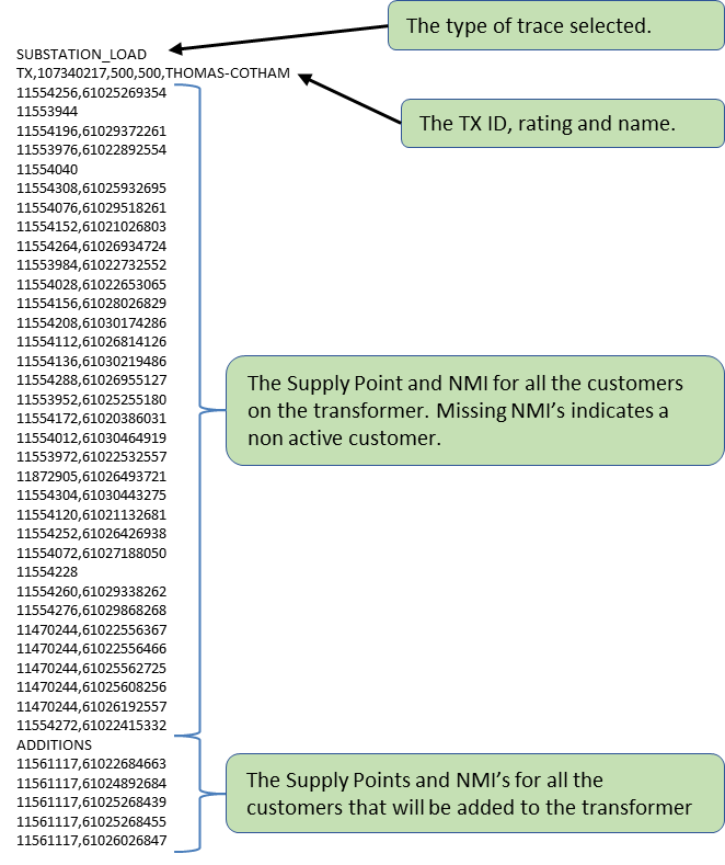
This can be generated by opening up any windows application, such as notepad, and pasting the clipboard.