Trend Displays
Maximum Demand
This landing page will bring up a blank trend display that will look something like this:
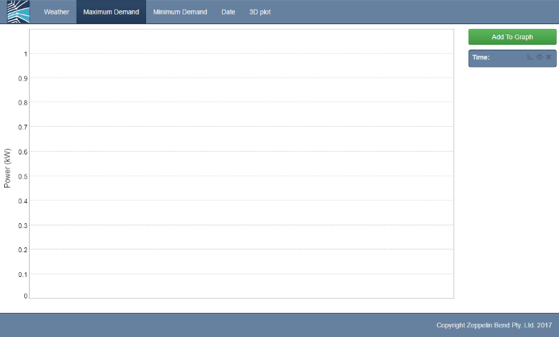
By default, the url places you on a landing page for getting an answer back on Maximum Demand.
Pressing the “Add to Graph” button will give you a dialog box where you can enter the name of a network asset where you want to find MD on.
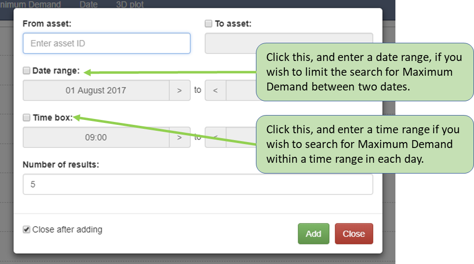
Start typing into the From asset edit box on the dialog. This will do an incremental search as you type, finding matching asset names.
The asset model used by the energy workbench is derived from the DMS. The names of the switches and circuit breakers in the DMS are sometimes inconsistent – this will be improved over time.
However, distribution transformer names adhere reliably to the names used by the OMS and HANA, so typing in the name of a transformer should return the results you are expecting.
Switches are usually found by entering the switch number followed by a G or an H, as in 40686 G…
Zone Substation Circuit breakers can be harder to find, however if you start typing in the zone name, you will normally get a list of assets to pick will feeder numbers. The DMS integration provides a reliable way to get Maximum Demand data for any part of the network, including HV Feeders.
Getting insights into load in the LV network is covered further in this document in section 3, Analysing Load Data with the GIS.
You can also enter a “To asset”. This allows you to find load between two assets. This only give back data if there is connected network between the assets, and may be better invoked from the DMS integration.
Lastly, you can limit the search for Maximum Demand to a date range, and time box the search so it only looks inside a time range for each day.
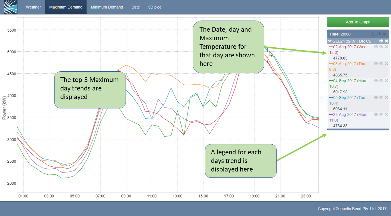
After picking an asset, and pressing “Add” – you should get something like the screen shot below.
Various additional options are provided in the trend legend, as explained below.
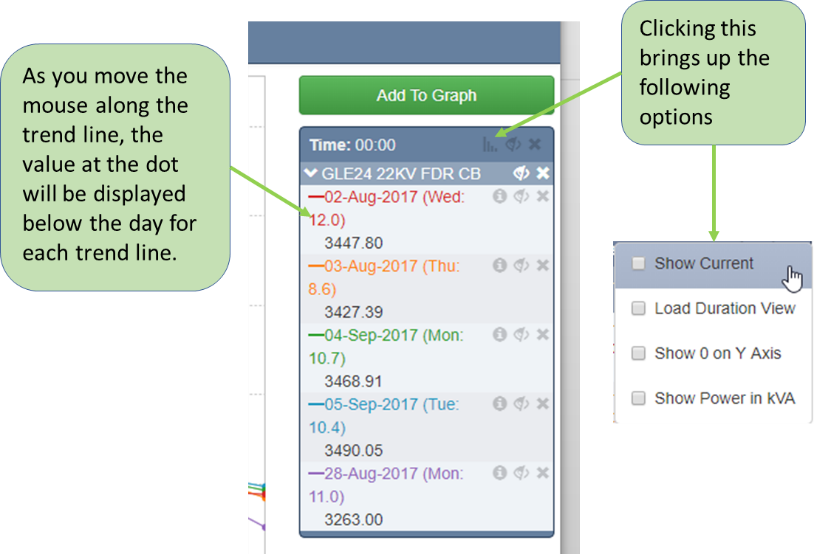
- Show Current – shows an approximation of the phase current.
- Load Duration View – shows how much relative time was spent at each load value.
- Show 0 on Y Axis – does exactly what it says.
- Show Power in KVA – it does this using an assumed power factor of 0.9
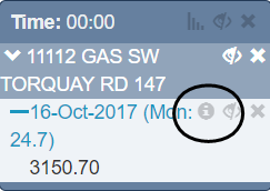
The “i” icon next to the date for the Maximum Demand allows you to bring up additional trend lines and information displays.
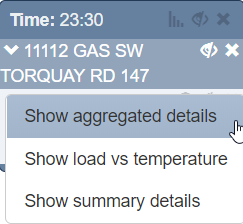
Show aggregated details displays a “drill down” showing all the assets for which load data was aggregated for the request.
In the case of a distribution transformer, the result will be the same – a single trend line.
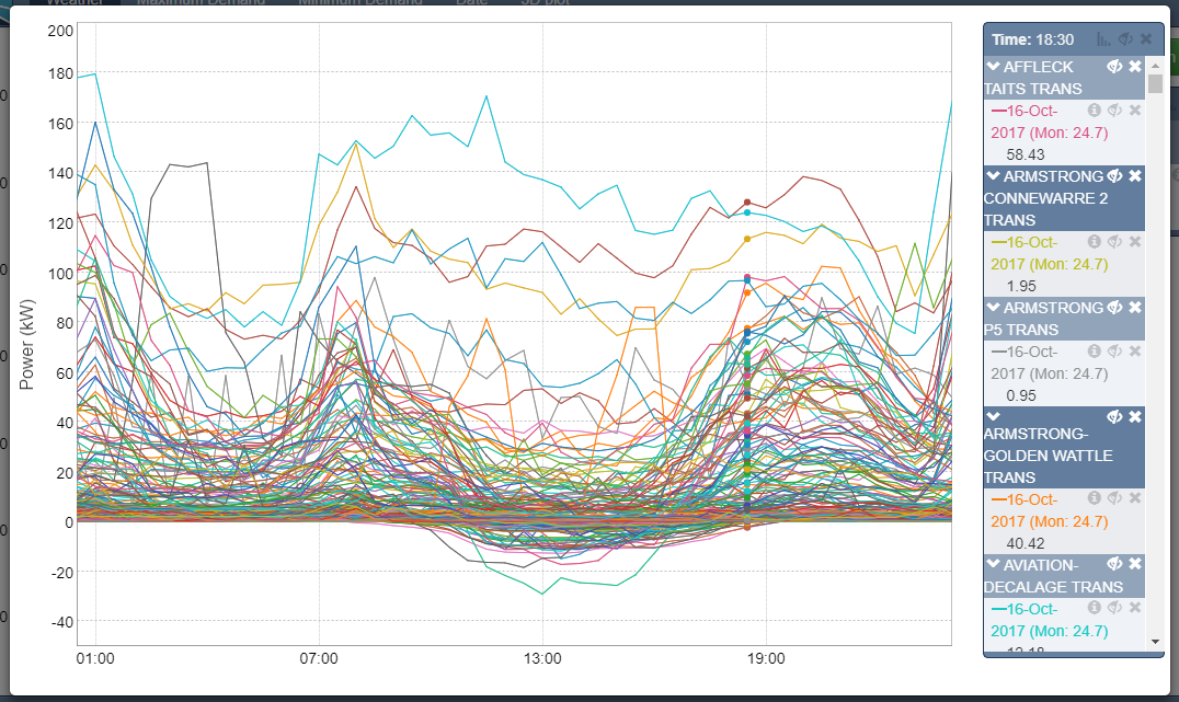
However for Maximum Demand requests performed on an asset that has multiple downstream load points, such as a switch or Circuit Breaker, a view of all the load that formed the aggregated, co-incident maximum demand trend line will be produced, as illustrated below.
The data behind this view may be exported to CSV format, and opened in Excel, by right clicking in the window and selecting the “Export to CSV” option.
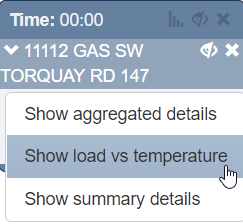
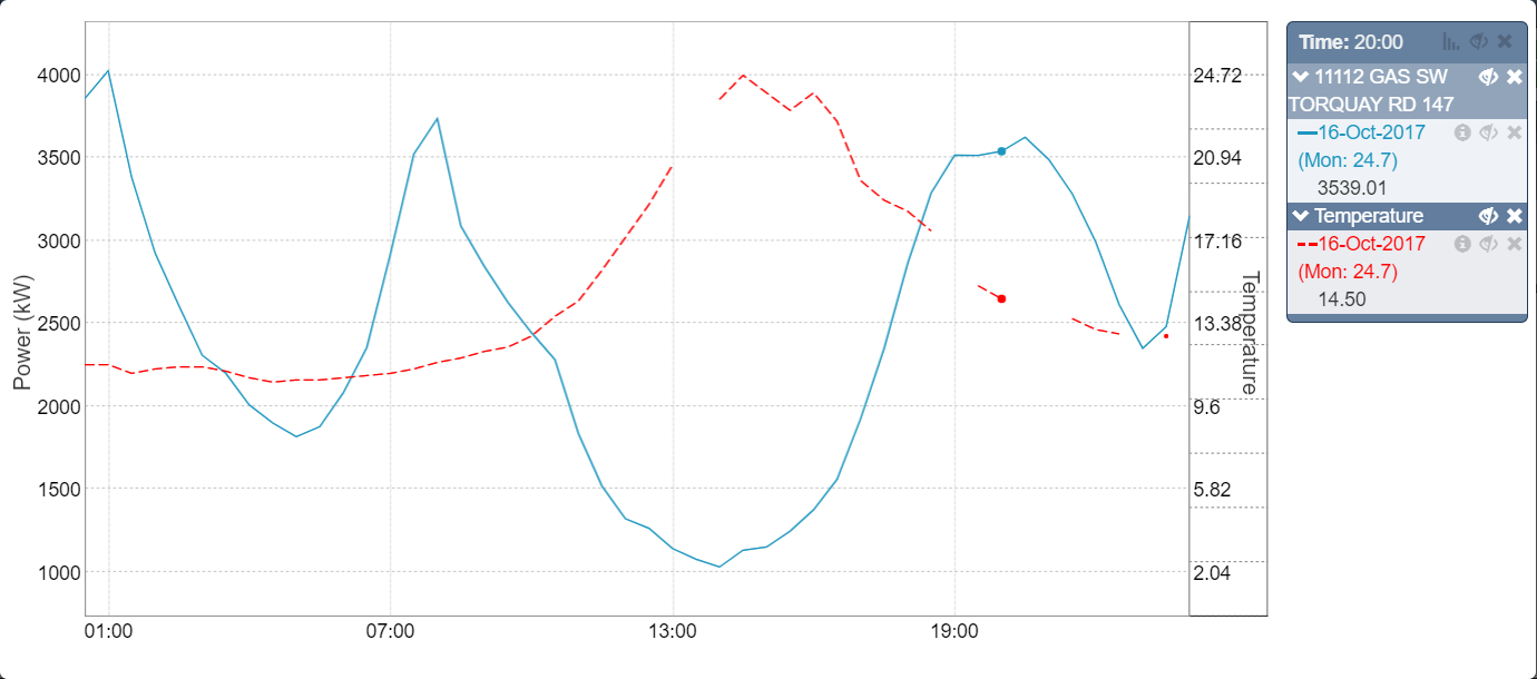
Show load vs temperature brings up a trend line showing temperature and load on the same trend display. The temperature is shown on the right hand axis (degree’s Celsius). An example is provided in the screen shot below. Missing data is shown as a break in the trend line.
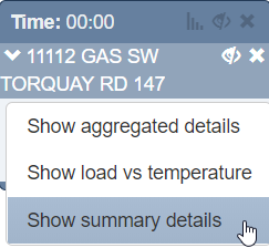
Show summary details brings up a text displays showing information about all the load points with non-zero loads included in the aggregation, and those with 0 load, and the maximum demand, day it occurred and highest temperature.
Additional menus along the top of the screen provide a way to look at additional load trends.
- Weather – allows historical load to be found for similar weather days.
- Minimum Demand – shows historical minimum demand load profiles.
- Date – shows load over a date range.
- 3D Plot – shown an x-y-z trend of load with time of day, and date as two of the axes, and load as the third axis.
Each of these is described in the following sections.
Weather Correlated Load

Load data from any point in the network, or between different, connected parts of the network, can be found for “similar” days in the past. The criteria for calculating a similar day is comprised of the following:
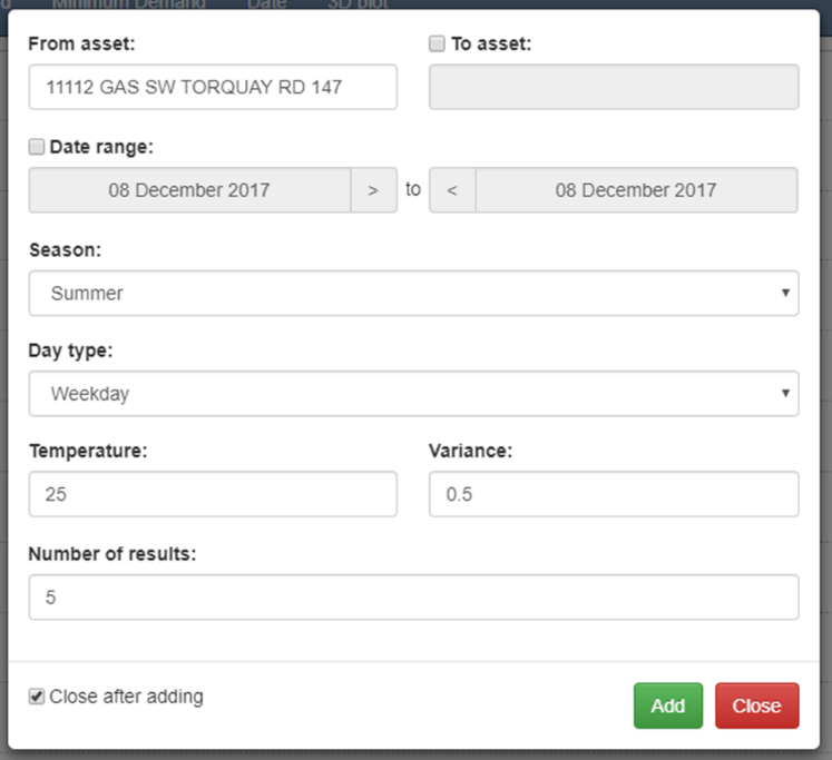
Season – only load data in Summer (October to March) or Winter (April to September), as selected, is considered.
Day Type – only load data that is on a Weekday, Saturday or Sunday, as selected, is considered.
Temperature – only load that occurs on a day with a maximum temperature plus or minus variance, as entered, is considered.
Date Range – only load that occurs within the selected date range is considered.
Pressing the Add button will give the same trend display as the Maximum Trend displays described above, except in this case the trend displays will represent the 5 closest correlated days to the criteria entered. If less than 5 days are found, only those will be displayed as trend lines.
Load Over A Date Range

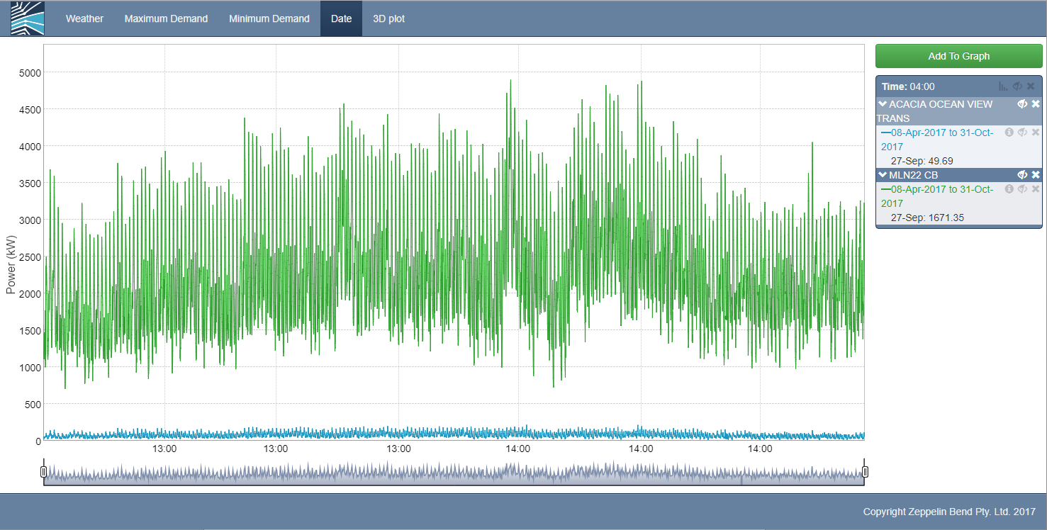
Load for downstream of any device, or between two devices, for a date range, can be trended by entering a date range, as illustrated below.
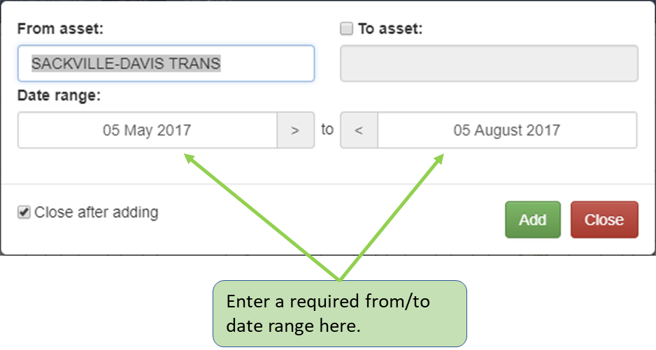
This will result in a trend line similar to the screen shot on the following page.

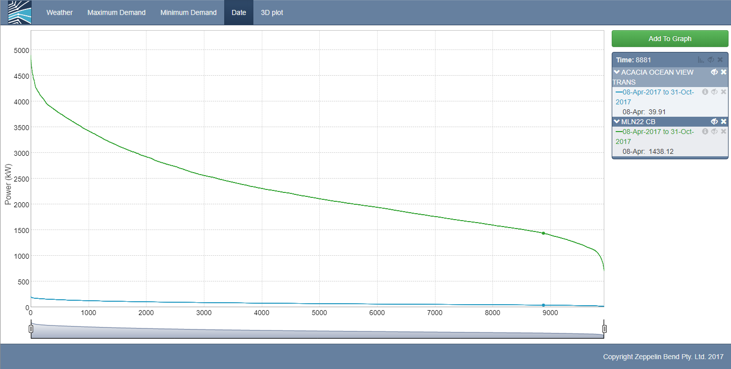
The load duration curve that can be invoked from the icon illustrated below can then be invoked to show the relative amount of time spent at each load.
This is illustrated below, where a classic load duration curve for a HV feeder is shown.
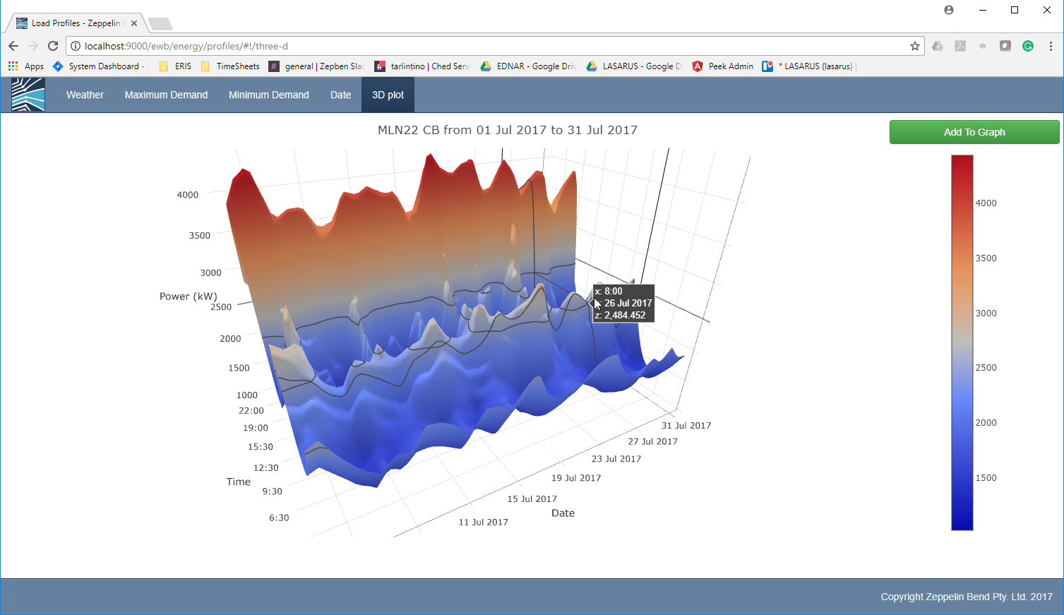
3D Plot

The 3D Plot produces a contour style plot with Power on the y axis, day on the x axis and time on the z axis.
As with the date range trend line, it is invoked by clicking “Add to Graph” and then supplying asset and date range information.
Clicking and moving the mouse on the contour will rotate the view. The intent of this visualisation is to allow anomalous behaviour over a time period to be readily identified.
Minimum Demand

The Minimum Demand function is identical to the Maximum Demand function in the way it is invoked and the options available from the trend line display. As the name suggests, it provides displays of the minimum n demand days for the selected asset.