What Are HCM Scenarios

HCM scenarios are named collections of input assumptions that define how distributed energy resources (DER) and demand growth will be distributed across the network in future years.

Why Scenarios Matter

Scenarios enable "what-if" analysis by allowing network operators to compare different DER adoption trajectories, test various technology mixes, and assess network constraints under different growth patterns. Rather than planning for a single predicted future, operators can explore multiple plausible futures and design networks that perform well across various conditions.

Data Architecture

HCM scenarios follow a hierarchical data structure that flows from detailed behavioural patterns up to high-level scenario definitions:

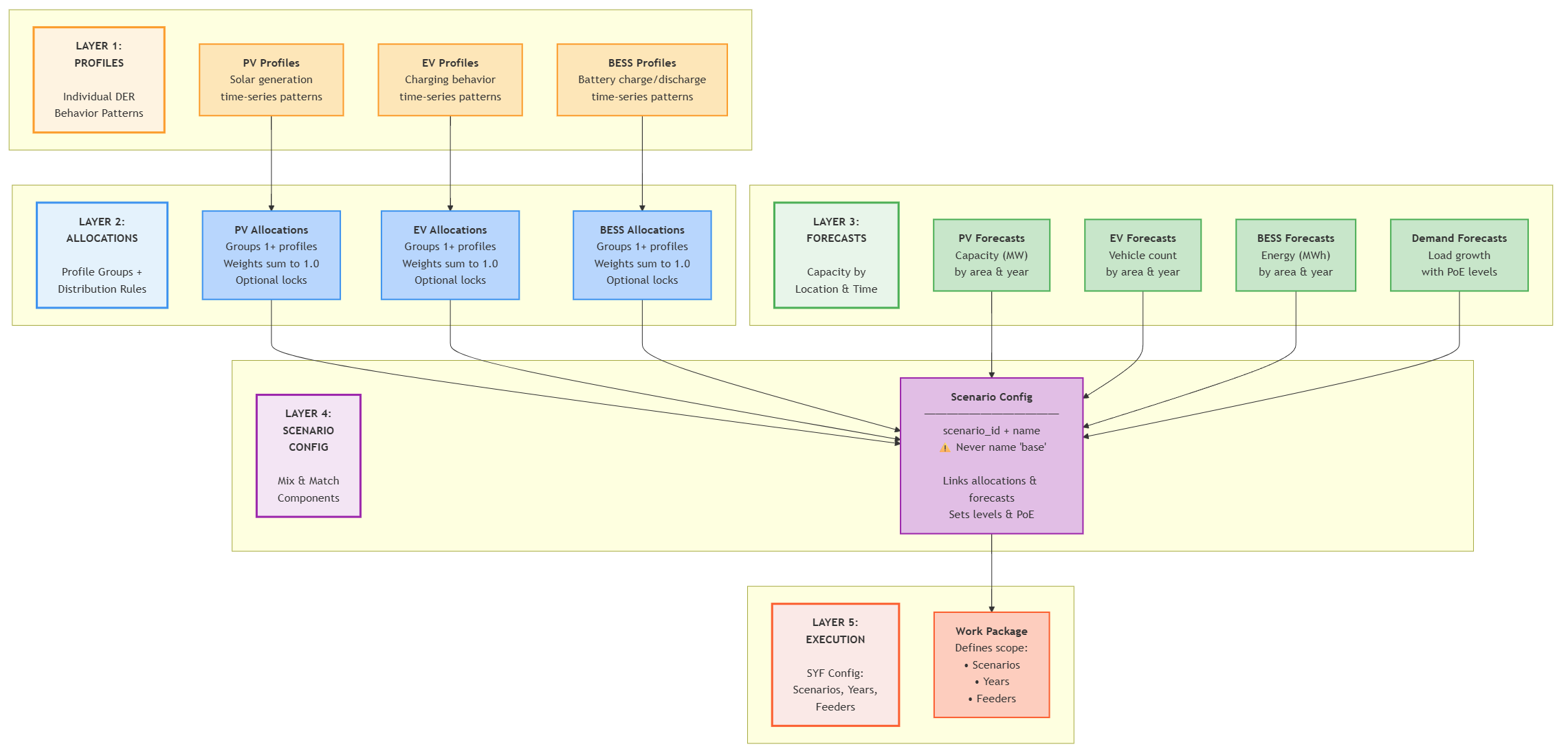
Profiles: Individual Behaviour Patterns

At the foundation are profiles - time-series data that capture how different DER technologies behave:

• PV Profiles define solar generation patterns with technical specifications like panel tilt, orientation, and inverter sizing
• EV Profiles capture charging patterns that vary by vehicle class, charger type, and usage patterns
• BESS Profiles model battery charge/discharge cycles with efficiency characteristics and control strategies

Each profile contains normalized power arrays (typically 17,520 intervals representing 30-minute data for a year) plus technical metadata about phases, capacity, and efficiency.

Allocations: Grouping with Rules

Allocations group multiple profiles for each DER type and define the rules for how they get distributed across the network:

• Probability weighting allows mixing different profile configurations (e.g., 60% of installations use 5 kW single-phase systems, 40% use 10 kW three-phase systems)
• Locking mechanisms control whether profiles can be used flexibly or must match specific years or feeders
• Probability weights are relative - they do not need to sum to 1.0, as only the proportions between them matter

Forecasts: Capacity by Location and Time

Forecasts specify how much DER capacity will be installed where and when:

• PV Forecasts define megawatts of solar capacity by network area and year
• EV Forecasts specify numbers of electric vehicles by class and location
• BESS Forecasts set storage targets in megawatts (inverter capacity) or megawatt-hours (storage capacity)
• Demand Forecasts project background load growth with probability of exceedance (PoE) levels

Forecasts are currently specified per feeder (FEEDER level).

Scenario Configuration: Mix and Match

Scenario configurations are where operators mix and match the building blocks above to create specific futures:

• Each scenario references specific allocation strategies for each DER type
• Scenarios can combine different forecast assumptions (high solar + low batteries, moderate EVs + high demand growth)
• Different scenarios can use different network aggregation levels and uncertainty assumptions

Profile Allocation Concepts

Profile allocation determines how behavioural patterns get distributed across network locations. Two key mechanisms control this distribution:

Probability Weighting enables realistic technology diversity. Instead of assuming all solar installations behave identically, allocations can specify that 60% follow one behavioural pattern while 40% follow another, representing different system sizes, orientations, or control strategies.

Locking Mechanisms control allocation flexibility:

• Year locking restricts profiles to specific time periods, useful for modelling technology evolution
• Feeder locking ensures location-specific characteristics are preserved, important for geographic differences

These mechanisms allow scenarios to balance computational efficiency with realistic representation of technology diversity across time and space.

"Existing" includes earlier forecast years

The steps below describe a single feeder in a single year. Existing or current PV, BESS or EV means everything on the feeder when that year's allocation starts. Under the default ADDITIVE strategy this includes DER added in earlier years of the same work package. See How scenarios evolve across years.

Consumers and NMIs

Allocation picks energy consumers but weights them by NMI: a consumer with several NMIs (e.g. an apartment building) gets one share of the candidate pool per NMI, capped at 10 for PV and 50 for BESS and EV. Upgrade thresholds apply per NMI, and existing DER on any of a consumer's NMIs counts. Consumers with no NMI receive no DER.

How PV is allocated in a scenario

Step 1: Check if the target is already met

The amount of PV needed for the year and feeder is extracted from the input table pv_forecasts, using pv_panel_capacity (MW, DC) whenever it is non-null (primary method), and falling back to inverter_capacity (MW, AC) only if pv_panel_capacity is null. The value of inverter_capacity has no bearing on which method is used - only the nullness of pv_panel_capacity matters. The total current PV capacity on the feeder is calculated by summing the ratings of all existing PV systems in the network model (in DC if using pv_panel_capacity and AC if using inverter_capacity).

The deficit is calculated as the difference between the forecast target and the current PV capacity on the feeder. If the deficit is zero or negative, no PV will be added and the process stops. No PV is ever removed, even if the forecast target is lower than current capacity.

Step 2: Build the initial candidate pool

The initial candidate pool gives each customer one share for each NMI without a PV system, so a single-NMI customer qualifies only if they have no existing solar. If the pool is empty, skip to Step 4.

Step 3: Select and install

A share is drawn at random from the candidate pool and that consumer is assigned a PV system drawn from a weighted profile pool. The profile determines system size and phase configuration (single or three-phase). The proportion of three-phase installs can be controlled via the max_percent_multiphase parameter. The share is then removed from the pool and the process repeats until either the target is met (then Steps 4 and 5 are not needed, so skip to Step 6) or the pool is exhausted (proceed to Step 4).

Step 4: Pool exhausted, target not met, add to customers with small existing system

If the forecast is not met using just customers without existing solar (e.g. every customer without existing solar has now been allocated a profile), then the candidate pool is rebuilt with customers whose existing PV is at or below pvUpgradeThreshold (default 5 kW) per NMI, with one share per NMI. The upgrade goes to the customer's smallest system. This captures installs that are small enough to be realistic upgrade/augmentation candidates.

• If new candidates are found, return to Step 3.
• If the pool is still empty, proceed to Step 5.

Step 5: Raise the upgrade threshold

If, after Steps 2-4, no candidates remain, the pool threshold is increased by 1 kW and the candidate pool is rebuilt - e.g. customers with up to 6 kW of PV per NMI are now considered candidates for receiving a new profile.

• If candidates are found, return to Step 3.
• Otherwise, repeat Step 5.

There is no upper bound on the threshold: allocation keeps raising it until the forecast target is met. This means commercial and industrial feeders, where systems well beyond residential sizes are normal, are allocated as forecast rather than being rejected. A large threshold is still reported, so an unrealistic forecast remains visible - see Allocation logs below.

The one case that is rejected is a profile pool where every profile has zero capacity. Since the target could never be reached, allocating such a profile fails the scenario with a MalformedScenarioException naming the PV target, rather than looping forever.

Step 6: Upgrading an existing system

Where a selected consumer already has a PV system, the new PV is attached to a separate scenario connection at that customer, with the inverter capacity and DC/AC ratio of the allocated profile. The existing system is not modified.

Note that if using the 'Advanced PV' feature, the new PV is compared against the cut-off using the forecast commissioning date, while the customer's existing PV keeps its own commissioning date.

How BESS is allocated in a scenario

Step 1: Check if the target is already met

The allocation target is extracted from bess_forecasts using whichever of capacity_mw (MW, AC, converted to VA internally) or capacity_mwh (MWh of storage) is set. Current BESS capacity is calculated by summing the AC inverter ratings (MW target) or rated storage (MWh target) of all existing battery systems on the feeder. For an MWh target, existing batteries with no rated storage count as 0 kWh.

If the deficit is zero or negative, the process stops. No BESS is ever removed, even if the forecast target is lower than current capacity.

Step 2: Build the initial candidate pool

Initial candidates are customers with a PV system with an inverter rating greater than 5 kVA. A customer gets one share per such PV system, up to one per NMI, less any batteries they already have. This reflects the real-world norm of BESS being paired with a reasonably sized solar installation. If no candidates exist the process skips to step 4.

Step 3: Select and install

A share is drawn at random and that consumer is assigned a BESS from a weighted profile pool, which determines system size and phase configuration. Three-phase installs can be capped via max_percent_multiphase in bess_forecasts (0.0–100.0). The share is removed from the pool and the process repeats until the target is met or the pool is exhausted.

Step 4: Pool exhausted, target not met

If the initial pool (Step 2) is empty, or becomes exhausted during Step 3, the pool is rebuilt dropping the PV co-location requirement. Every consumer whose existing BESS is at or below bessUpgradeThreshold per NMI (default 5000, in VA for an MW target or Wh for an MWh target) gets one share per NMI, including consumers with no battery. A consumer with fewer batteries than NMIs gets a new system; otherwise its smallest battery is upgraded.

• If new candidates are found, return to Step 3.
• If still empty, proceed to Step 5.

Step 5: Raise the upgrade threshold

The threshold is raised by 1 kVA (or 1 kWh for an MWh target) and the pool is rebuilt.

• If candidates are found, return to Step 3.
• Otherwise, repeat Step 5.

As with PV, there is no upper bound on the threshold - allocation continues until the forecast target is met, and the growing threshold is reported in the logs (see Allocation logs below). A profile pool containing only zero capacity profiles fails the scenario with a MalformedScenarioException naming the BESS target.

Step 6: Upgrading an existing system

Where a selected consumer already has a BESS, the new BESS is attached to a separate scenario connection at that customer, with the inverter capacity and storage capacity of the allocated profile. The existing system is not modified.

How EV is allocated in a scenario

Step 1: Check if the target is already met

The allocation target is extracted from ev_forecasts using number_of_ev. The forecast column accepts decimals, but HCM currently reads the value as an integer, so any fractional part is truncated (e.g. 5.7 becomes 5). Current EV charger count is calculated by summing all existing EV charging units on the feeder.

If the deficit is zero or negative, the process stops. No EV chargers are ever removed, even if the forecast target is lower than the current count.

Step 2: Build the candidate pool

Each consumer gets one share per NMI, capped at 50. Shares are handed out in rounds, so no consumer gets a second charger per NMI until every consumer has one per NMI, counting chargers added in earlier years. If no consumers exist, a warning is logged and the process stops.

Unlike PV and BESS, there is no upgrade path for EV - existing charger data is not currently available at the level of detail required for upgrade modelling, so all installations are treated as new.

Step 3: Select and install

A share is drawn at random and that consumer is assigned an EV charger from a weighted profile pool, which determines charger size and phase configuration. Three-phase installs can be capped via max_percent_multiphase in ev_forecasts (0.0–100.0). Each charger always receives its own new connection, and the same consumer can receive multiple chargers. The process repeats until the target count is met. The EV chargers added are logged by total count and total kW.

There is no limit on the number of chargers a single consumer can receive. Instead, if the target works out to at least one charger per NMI on the feeder, a warning is logged before allocation starts (see Allocation logs).

How demand scaling is applied

Demand Scaling is meant to represent the increase in load from general load growth, electrification, urban infill/densification, new appliances etc. It takes the loads of a given feeder and scales them by a ratio. It is not time varying, all loads across the year will be increased by the same ratio.

Unlike DER allocation, which targets an exact forecast quantity, demand scaling applies a growth ratio derived from the forecast to each base load in the model. The model does not re-anchor loads to match the forecast's absolute magnitude - it only applies the relative change between the base year and the target year.

Note: When getting the customer loadshapes from the cpi_aggregations, the loadshapes are split into import and export, and demand scaling only applies to imports (i.e. loads), and not exports. Exports are never scaled; they are instead augmented by adding PV/BESS, see above.

Step 1: Determine the base year

The base year for demand forecasting purposes is the year of the final interval of the load data time period selected.

note

Intervals are time-ending (see time conventions) and end_time is exclusive, so a full calendar year is:

start_time  =   2025-01-01T00:30
end_time    =   2026-01-01T00:30

This covers all of 2025, and the base demand year will be 2025.

Step 2: Determine the seasonal peak timestamp

The load database is used to determine the timestamp of the feeder's annual peak. This timestamp is used to select the correct seasonal forecast (winter or non-winter), since many DNSPs maintain separate demand forecasts for summer and winter peaks. Real and reactive load are handled independently, each using their own seasonal peak timestamp.

Note: the peak timestamp itself is identified from net load (imports minus exports), not imports alone. This only affects which timestamp is used to pick the winter/non-winter forecast - the scaling factor is still applied to imports only (see above).

Step 3: Calculate the scaling factor

For each feeder, HCM fetches the forecast total demand for both the base year and the target year, then computes:

scaling_factor = forecast_target_year_peak / forecast_base_year_peak

Both the base year and target year peaks come from the forecast input database, not from measured load data. This is intentional: using forecast values for both sides of the ratio ensures consistency, since the growth trend is derived entirely from the forecaster's assumptions rather than mixing actuals with projections.

warning

Demand scaling fails silently in two cases - the scaling factor defaults to 1.0 (no scaling applied) and only a warning is logged, with no error raised:

• The scenario has no demand forecast configured at all.
• A forecast row is missing for the feeder/year/season combination needed to compute the ratio.

If a feeder's load isn't growing as expected in a scenario, check the logs for these warnings before assuming the forecast data is correct.

Step 4: Apply the scaling factor

The scaling factor is applied to each customer's base load (imports only) to produce the scaled load for the target year.

Example

Consider a feeder with three customers, each with a smart meter. In the base year (2026), their measured loads are:

Customer	Base load
A	80 kW
B	120 kW
C	150 kW

The total base load in the model is 350 kW. However, the demand forecast puts the feeder at 500 kW in 2026, growing to 600 kW in 2027, a scaling factor of 1.2.

In the 2027 simulation, each customer's load is scaled by 1.2:

Customer	Base load	Scaled load (2027)
A	80 kW	96 kW
B	120 kW	144 kW
C	150 kW	180 kW

The total modelled load becomes 420 kW - not the 600 kW the forecast projects. The 150 kW gap between the model's base load (350 kW) and the forecast base year (500 kW) is preserved and carried forward. HCM has no mechanism to close this gap; it only applies the growth ratio.

What this means in practice

If a feeder's base loads are understated relative to the forecast starting point - for example because some customers lack smart meters and are represented by default profiles - the scaled loads will remain understated by the same proportion throughout the forecast period. This does not affect DER allocation, which still targets the full forecast quantity. As a result, the apparent impact of DER on the feeder may look larger than it would in reality, since the DER load is being added on top of an already-understated baseline.

Allocation logs

Because the upgrade threshold is unbounded, the logs are the way to tell an unusually large but legitimate forecast from a misconfigured one.

Each time the threshold crosses another 10 kW (at 10 kW, 20 kW, 30 kW and so on) a warning is logged naming the threshold reached and the forecast target that is driving it:

The whole feeder is now allocated with >=20kw systems per NMI and this risks non-convergence. Is your forecast scenario meant to be this large: 4.5E7? Will continue allocating until the forecast is met.

The equivalent BESS warning names the BESS target instead. For an MWh target it steps in 10 kWh, with the target in Wh. Treat these as a prompt to sanity-check the forecast row for that feeder and year, not as an error: allocation carries on regardless. The higher the threshold climbs, the more the resulting model is dominated by large upgraded systems, and the greater the chance the power flow fails to converge.

Each individual threshold increase is logged at DEBUG by the model generator, reporting the capacity allocated so far, the new threshold, and how many consumers became viable for upgrade. Run the generator at DEBUG level to see the full progression when investigating a scenario that allocated much larger systems than expected.

For EV, the target is known up front, so a single warning is logged before allocation when the target is at least one charger per NMI:

Target of 1200 EV chargers is 1.5 chargers per NMI across 800 NMIs, which may risk non-convergence. Check the forecast scenario is meant to be this large.

An info log after allocation reports the number of chargers and total kW added. As with PV and BESS, allocation carries on regardless.

A scenario that is genuinely unallocatable - a profile pool where every profile has zero capacity - fails with a MalformedScenarioException naming the target that could never be met.

How scenarios evolve across years

A work package usually models several forecast years for each scenario. How each year's model relates to the one before it is set by feederScenarioAllocationStrategy in the Model Config. There are two strategies: ADDITIVE (the default) and RANDOM.

Additive allocation (default)

With ADDITIVE, the years for each feeder and scenario are built in sequence, earliest first. Each year starts from the previous year's model, including all the DER that scenario allocation added in earlier years, and only adds what is needed to close the gap to that year's forecast.

Example

A feeder has 1.6 MW of PV in the network model. The PV forecast for the scenario is 2.0 MW in 2026, 2.5 MW in 2027 and 2.4 MW in 2028.

Year	Forecast	Existing at start of year	Deficit	Added this year	Total in model
2026	2.0 MW	1.6 MW (network model)	0.4 MW	0.4 MW	2.0 MW
2027	2.5 MW	2.0 MW (incl. 2026 additions)	0.5 MW	0.5 MW	2.5 MW
2028	2.4 MW	2.5 MW	-0.1 MW	Nothing	2.5 MW

In 2027 the customers who received PV in 2026 keep it and are no longer in the "no existing solar" candidate pool, so the additional 0.5 MW goes to different customers.

What this means in practice

• DER stays where it was placed. A customer allocated PV, BESS or an EV charger in one year keeps it in every later year. Constraints therefore develop in the same locations over time, which makes year-on-year comparisons for a zone meaningful.
• Candidate pools shrink each year. Because earlier allocations count as existing DER, the pool of customers without PV gets smaller every year. On feeders with high forecast uptake, later years are more likely to run out of new candidates and move on to upgrading existing systems (PV and BESS Step 4 onwards), which raises the chance of the allocation log warnings.
• Earlier PV allocations affect BESS candidates. The initial BESS pool favours customers with a PV system above 5 kVA, and this includes PV allocated in earlier years. PV is allocated before BESS within each year, so PV added in the same year counts too.
• Falling forecasts are not reflected. No allocated DER is ever removed, so where a forecast decreases, the model holds the highest level reached so far.
• EV counts are cumulative too. The EV target for each year is compared with the chargers already on the feeder, including those added in earlier years.
• A year depends on the years modelled before it. A year modelled on its own does not produce the same allocation as the same year modelled after earlier years, even with the same seed. Do not compare, for example, 2030 from a work package covering only {2030} with 2030 from one covering {2026, ..., 2030} and expect identical DER placement.
• Model a contiguous block of years. Only the listed years are modelled, so for {2026, 2030} the 2030 model builds directly on 2026. Intervention work packages require single or contiguous years for this reason, see Interventions.

The link_to_input output table reports the DER added by scenario allocation for each measurement zone as a cumulative total up to and including each year, not the amount added in that year.

Demand scaling is not cumulative

Demand scaling does not build on the previous year in the same way. Each year's scaling factor is calculated directly from the forecast base year to that target year (see How demand scaling is applied), so a year's load is the same whether it is modelled on its own or after earlier years. Only DER allocation carries state from one year to the next.

Random allocation

With RANDOM, each year is allocated independently, starting from the original network model rather than the previous year's model. Each year's DER placement is unrelated to the other years, so a customer can have scenario PV in 2027 and none in 2028, and constraints can move between zones from year to year purely because of where DER happened to be placed.

RANDOM is not supported for candidate-based interventions: the work package fails to build. See How to run an Intervention Work Package.

Reproducibility and seeds

Customer selection and profile selection are random. The seed parameter in the Model Config controls this randomness:

• seed not set (default): a new random allocation is generated for each run. Two otherwise identical work packages can place DER on different customers. Feeder totals still match the forecast, but zone-level results can differ between the two runs.
• seed set: re-running with the same seed and the same inputs (network model, feeders, scenarios, years, forecasts, profiles and allocation configuration) produces the same allocation.

Use the same seed for parent and intervention work packages

When comparing an intervention work package with its parent, both must use the same seed, as well as the same years and other configuration. Otherwise DER is placed on different customers in the two runs, and differences in the results may come from the change in allocation rather than the intervention. See Checking the work packages are comparable.

Scenario Execution

Scenarios run independently within work packages. Each scenario has its own allocation sequence, so DER placement in one scenario does not affect another.

For step-by-step guidance on configuring scenarios, see the How to Configure HCM Scenarios guide.

warning

Never name a custom scenario base. Regardless of the contents of the scenario_configuration input table, you can always run a base scenario, which represents current network conditions without additional DER uptake or demand changes. Naming your own scenario base will cause conflicts with this system baseline.