Trends
The Load trends tab is on the right hand panel.
Load Trends Tab
Load Trends show time series aggregated smart meter data for any part of the distribution network. The following types of trend displays are available:
- Daily profiles of the top 'n' max/min days,
- Load over time, and
- Load duration.
The load can be expressed in kW, kVAr, kVA or, for conductors, Amps.
When combined with rating information for conductors and transformers, it's possible to easily identify overloaded assets of this type anywhere in the network.
Load trends and tracing are related - a load trend is created by tracing out the network and aggregating the load of customers connected to the traced network. Whenever a load trend is created, it will have a corresponding trace. The colour of the pen lines on the load trend will have the same colour as the traced network on the map corresponding to the trend, making it easy to visualise the part of the network the load trend applies to.
How They Work
Load trends are generally only available in the Network Explorer if your organisation has complete, or nearly complete, smart meter penetration and 30 minute interval (or less) power or energy data, and this is made available from the meter data management system for ingestion by the Energy Workbench.
The load trends are calculated by summating all smart meter load data connected to assets that form part of an isolation or downstream trace, for the number of days needed to satisfy the type of trend requested. For a max/min trend display, this will be all available historical data, unless a From-To date range is selected, which will limit the search to the days in the specified From-To date. For load-over-time and load duration trends, all smart meter data in each day in the specified From-To date range will be summated.
In the Energy Workbench, the interval between smart meter load data samples is 30 minutes, with Max/Min and date range trend displays drawing a straight line between each 30 minute load data point to form a continuous trend line. Each data point represents the summated load at that sample time for all smart meters connected to customers found in the downstream trace. To improve responsiveness, the load data for all customers connected to transformers is pre-aggregated for each 30 minute sample interval, so that load requests in the HV network will use the aggregated load values for the transformer, rather than tracing into the LV network and looking for smart meter load data on individual customers.
This aggregated load can be cached in memory, depending on how the Energy Workbench has been deployed for your organisation. When this is done, the load trends will be very performant for trends in the HV network - returning most results in a few seconds. If the load data is not cached in memory, the results can take a lot longer to be returned.
When a load trend is requested on any of the LV network, only the load data on that portion of the LV network that is traced will be included. The individual load points cannot be cached in memory as the amount of memory that would be required would be too large in practical terms, and so load trend requests for LV only network can take somewhat longer than the HV load requests that can use the in-memory cache. For this reason, limiting the date range of these trends to days of interest is highly recommended.
Smart meters typically report real energy values for each interval in kilowatt hours (kWh). Energy is expressed in kilowatt hours, so for a 30 minute energy reading (half of one hour) the average power (kW) for that 30 minute interval can be found by multiplying the energy by 2. The Power Factor for individual smart meters is generally not available, and so the real power (kVA) is calculated by multiplying the real power (kW) by a user entered power factor. When dealing with conductors, the current is calculated using the number of phases present on the conductor and the operating voltage.
Invoking a Load Trend.
Load trends are invoked from an icon on the pop up menu for each asset, or alternatively from an icon in the trace panel for isolation and downstream traces. When the trend is invoked, the right hand screen panel will open, showing the trend tab. This panel can be resized by dragging the left hand panel edge left or right. The default trend displayed is the "Max/Min" trend. This can be changed to a "Date Range" trend by selecting this option in the "Mode" drop down.
More than one trend can be compared concurrently on the same axis by selecting multiple traces from the "Selected Traces" list. This is explained in more detail below.
Max/Min Trends
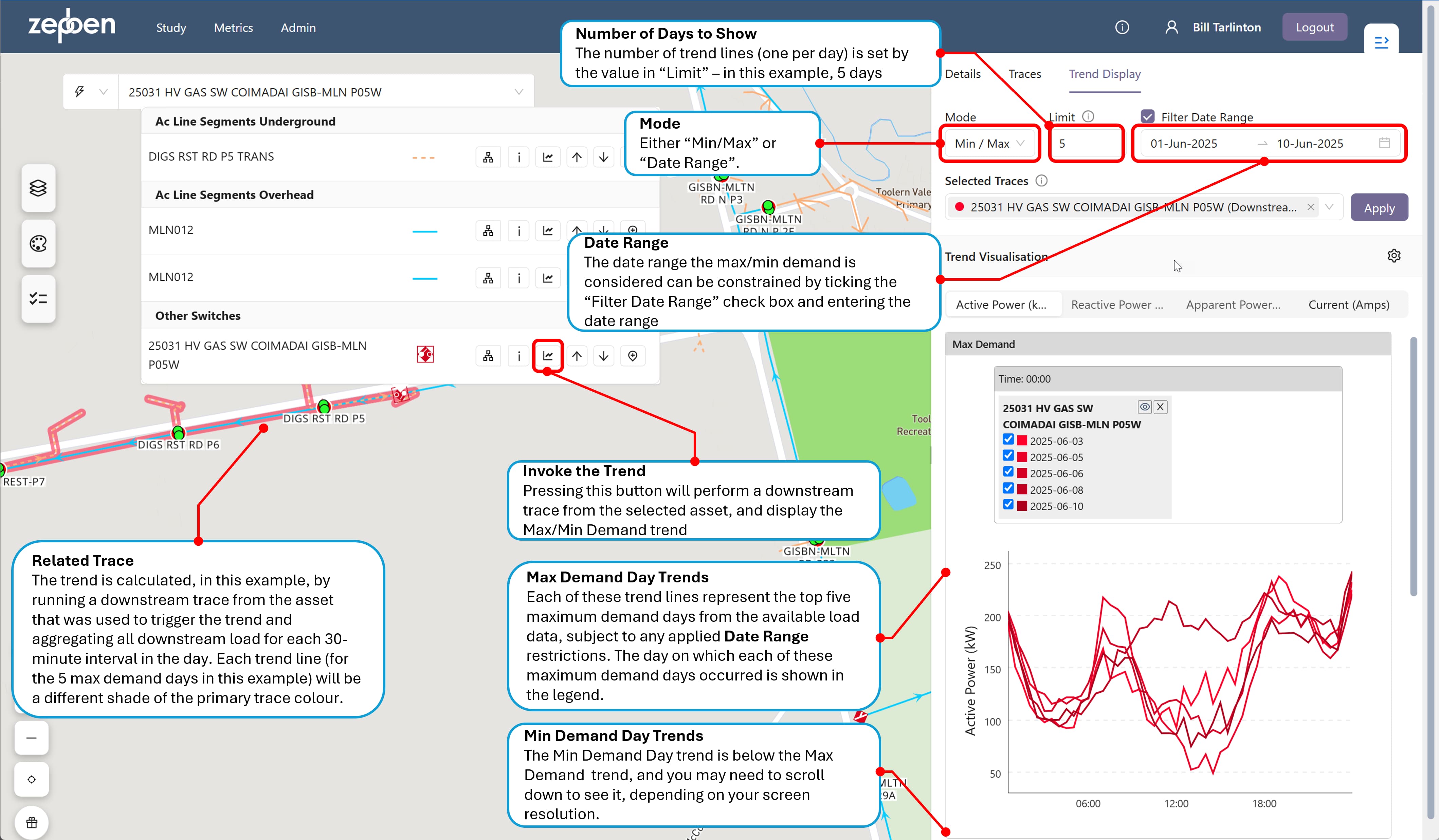
This shows a set of 'n' trend lines for a 24 hour period. The number of trend lines shown will be the number specified in the "Limit", with the default number being 5. The x axis of the trend represents a 24 hour time period, with 48 intervals - each one representing the average load for the previous 30 minute time slot.
The algorithm to determine the maximum and minimum load days ranks each day in the historical date range being considered according to the highest load value of the aggregated smart meter data for that day - the peak value. The maximum demand days are the days with maximum peak value within the day. The minimum demand days are the days with the lowest peak values within the day.
Each trend line on the "Max Demand" graph represents one of the top 'n' maximum demand load days. Each trend line on the "Min Demand" graph represents one of the 'n' minimum demand load days.
If a "From" and "To" date is not provided, all available days with load data in the past will be considered.
The screen shot below shows a Max/Min load trend that has been invoked from a switch.
Date Range Trends
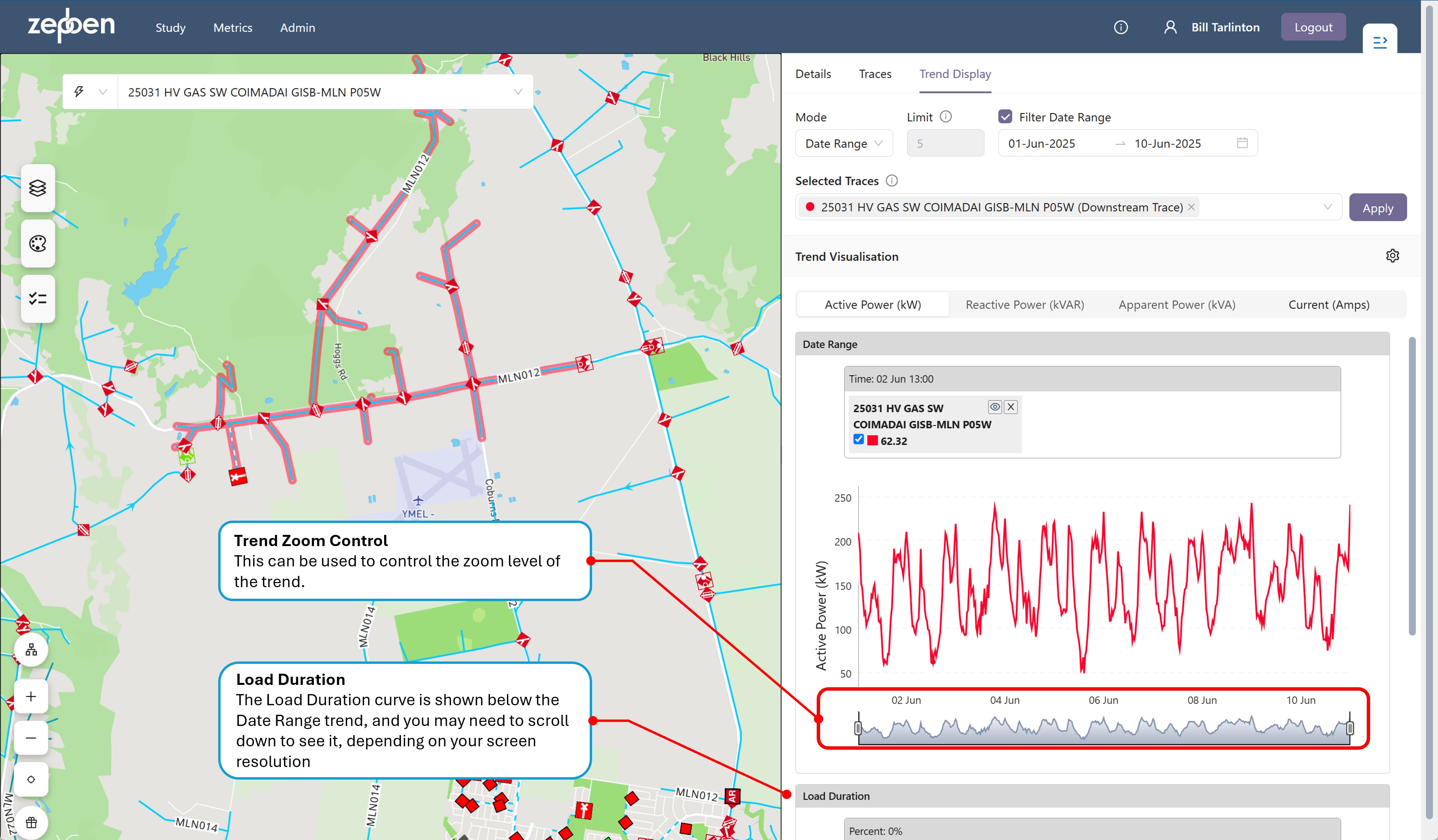
As the name suggests, a date range trend provides a continuous load trend for assets within a downstream or isolation trace, for the specified date range. As with the Max/Min trend, the load can be expressed in kVA, kVAR or kW for all assets, and for conductors, it can also be expressed in Amps, using the operating voltage and phases present of the conductor.
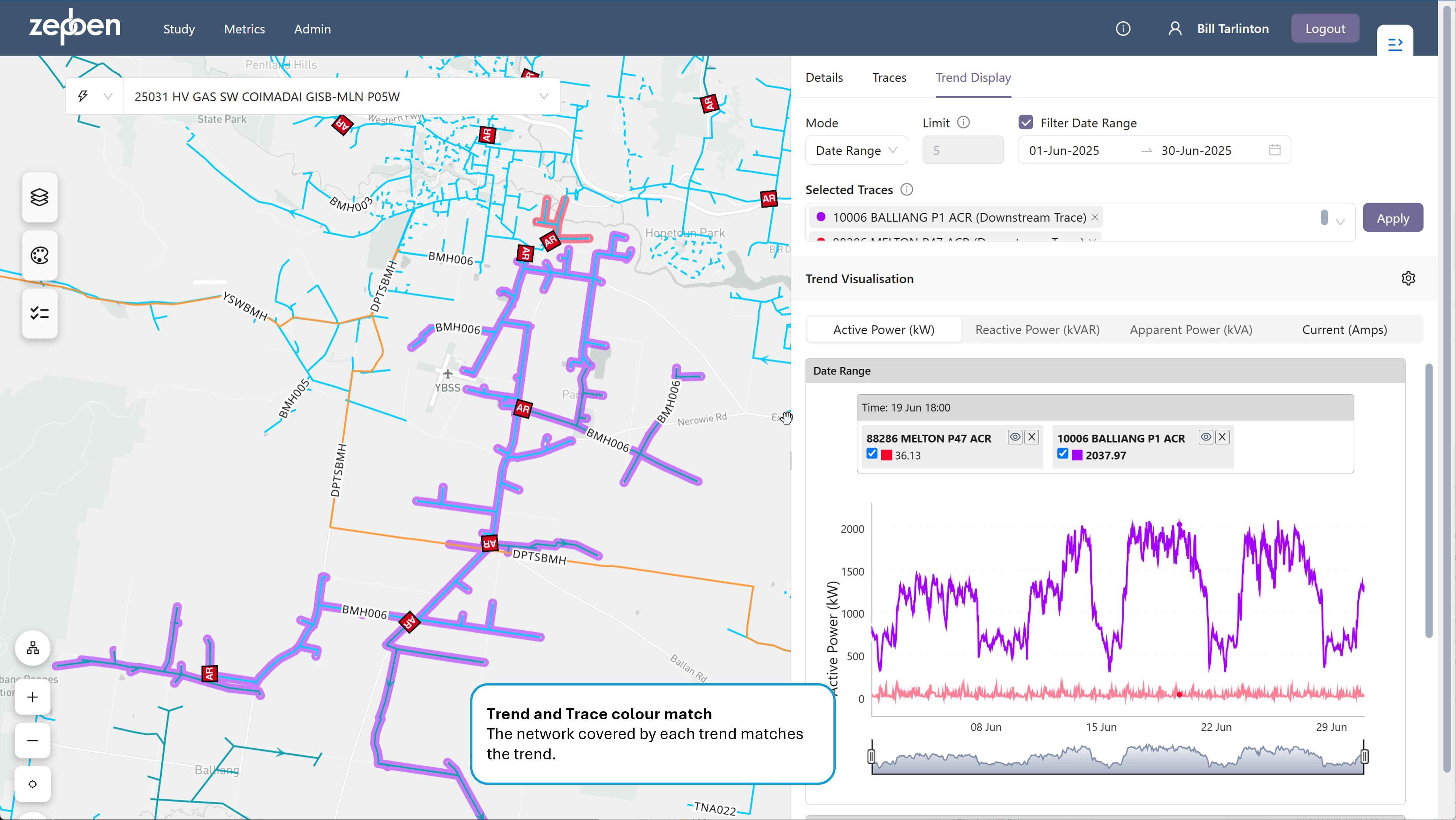
The pen colour of the trend can be changed by changing the colour of its corresponding trace in the "Traces" tab of the right hand panel. The pen colour of the trend follows the colour of the trace on the map, allowing you to easily understand which part of the network is covered by the trend.
A typical date range trend is provided in the illustration below.
In some cases, there will be gaps in the trend display - this indicates there is no data available for those dates. This can happen because either there was no smart meter data available, or because some days have been removed from the historical record by your system administrator for performance and storage reasons, as they did not have any load that was "of interest" to most people, that is, not a high or low demand day.
Load trends of aggregated smart meter data should in theory be close to the values reported by SCADA or other forms of telemetry - however in practice there may be missing smart meter data for a portion of the network being examined, or there can be mapping issues between the smart meter data and the GIS supply points they connect to. For this reason, its always a good idea to compare the load data from other telemetered sources too ensure the smart meter trends are providing acceptably accurate results. Once that is done, you can be reasonably confident the load trends will give you accurate data anywhere along the feeder.
The aggregated smart meter trends are always provided against the networks normal state. This means if you are comparing, for instance, a load value obtained from SCADA with a load trend in the network explorer obtained from smart meter data, and the network was in an abnormal switched state at the time, you will see differences in the load trends. The smart meter derived trends effectively remove the impact of changing switch states in the network.
Real and Reactive Power, and Current
Additional tabs allow for the display of trends of Reactive Power, Apparent Power and Current. These will only provide trend lines if either
- Reactive power is supplied by the Energy Workbench server for each time interval, or
- A default power factor is supplied.
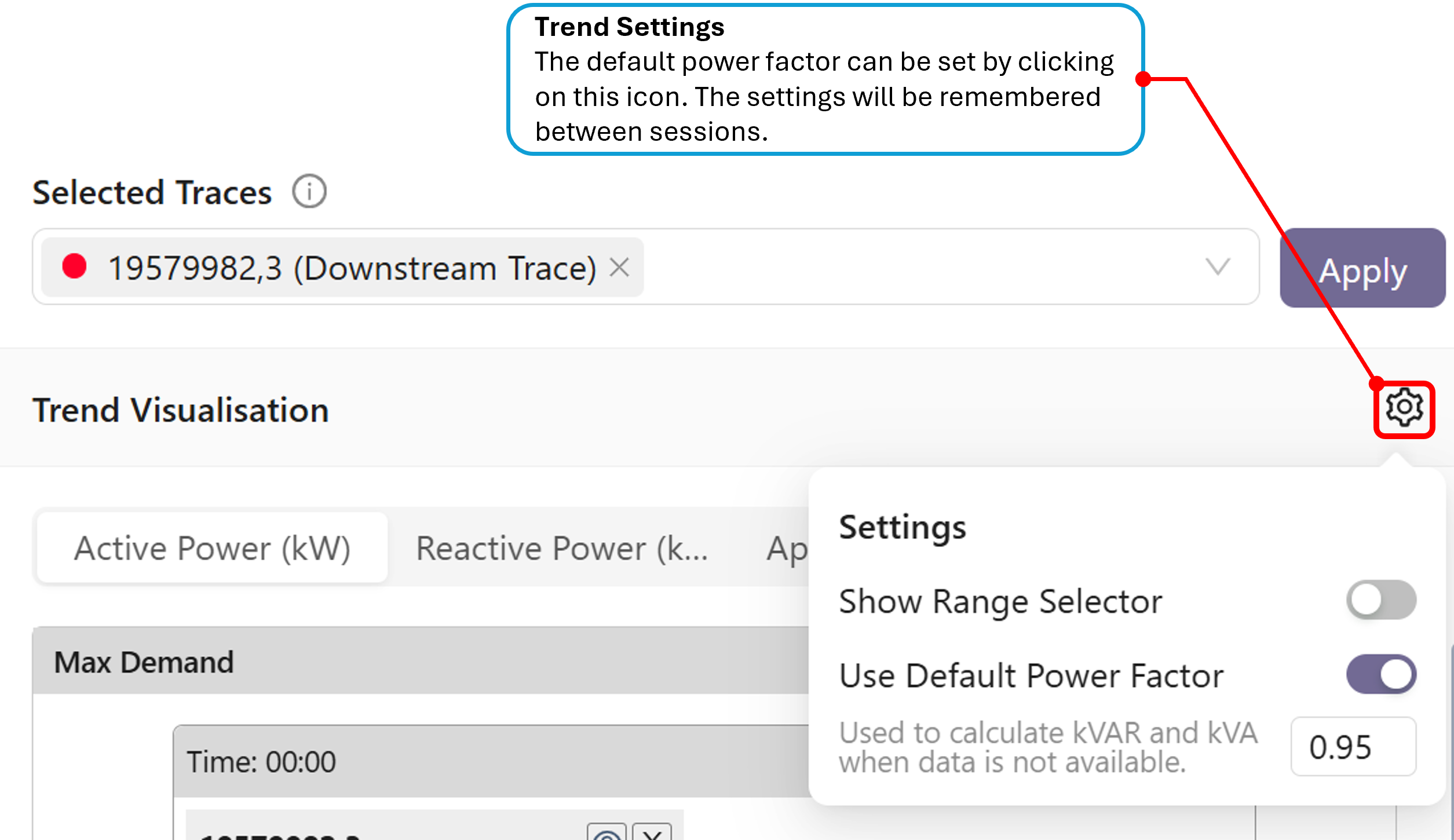
The default power factor can be entered via "Trend Settings", as illustrated in the screen shot below. If this setting is used, any missing reactive power in a time slot supplied by the Energy Workbench will be filled by applying the user supplied power factor to the real (Active) power. It will not overwrite any reactive power supplied by the Energy Workbench.
Ratings Trend Lines
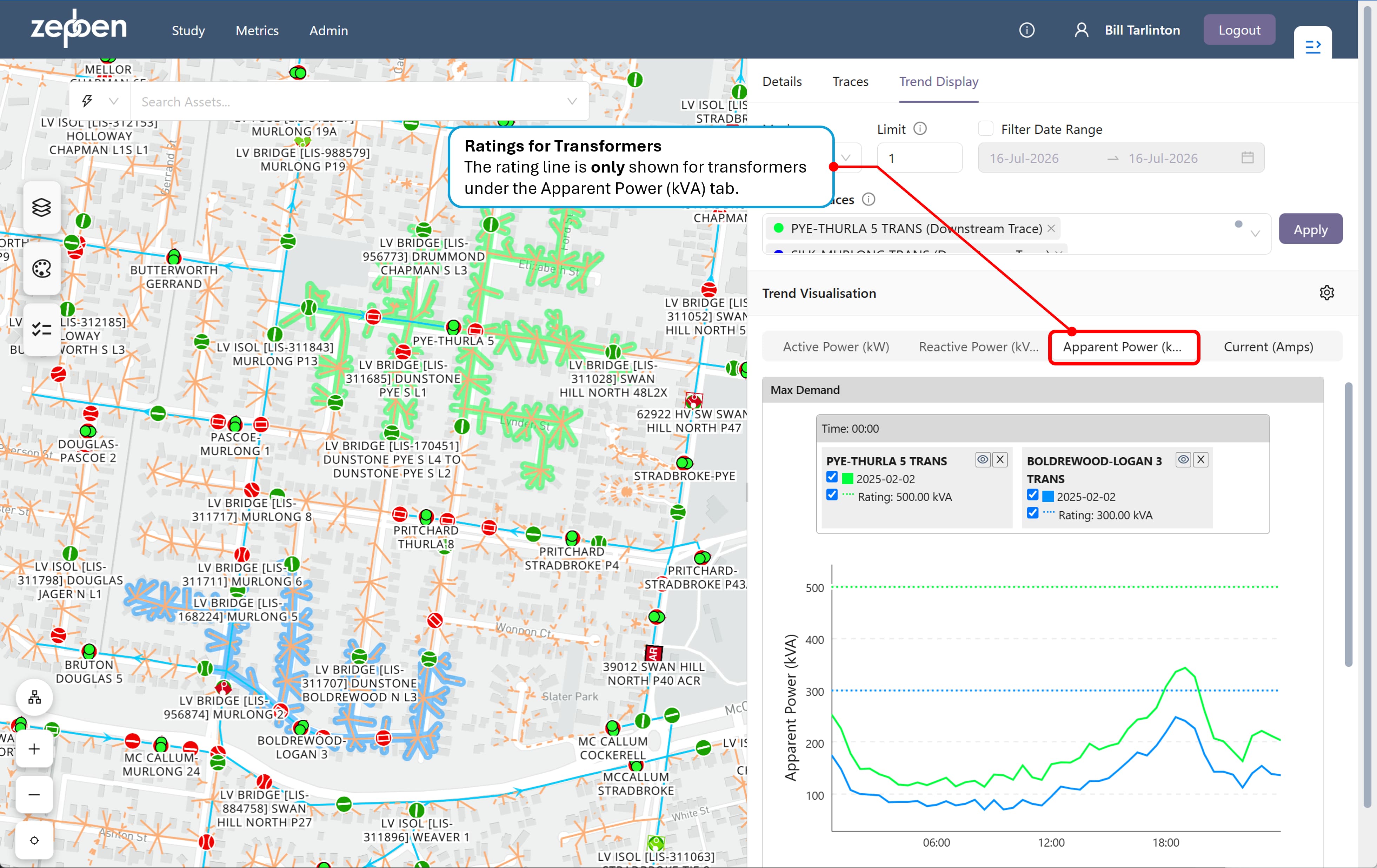
A rating trend line will be shown for transformers and conductors, where the rating is available.
In the case of transformers, the rating line will only be shown on the Apparent Power(kVA) tab, because transformer ratings are expressed in kVA.
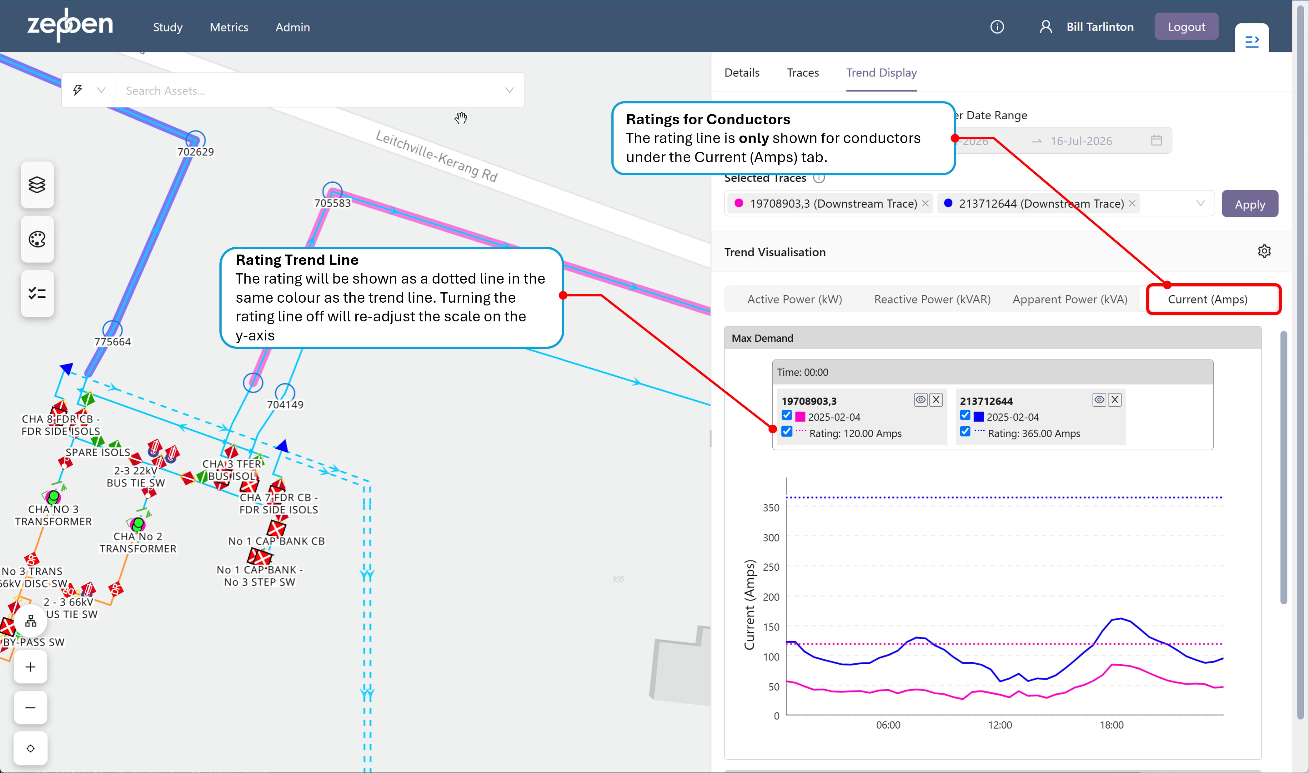
In the case of conductors, the rating line will only be shown on the Current(Amps) tab, because conductor ratings are expressed in Amps. The current is calculated taking into consideration the operating voltage and phasing of the conductor.
The screen shot below shows two maximum demand load trends, with a single value of maximum demand for each conductor, and showing the ratings for each.
The calculation of Current is only as good as the accuracy of the underlying network model - if the operating voltage or phase is not correct, the trend line for Current will be incorrect
The screen shot below shows two maximum demand load trends, with a single value of maximum demand for each transformer, and showing the ratings for each.
Load Duration Curves
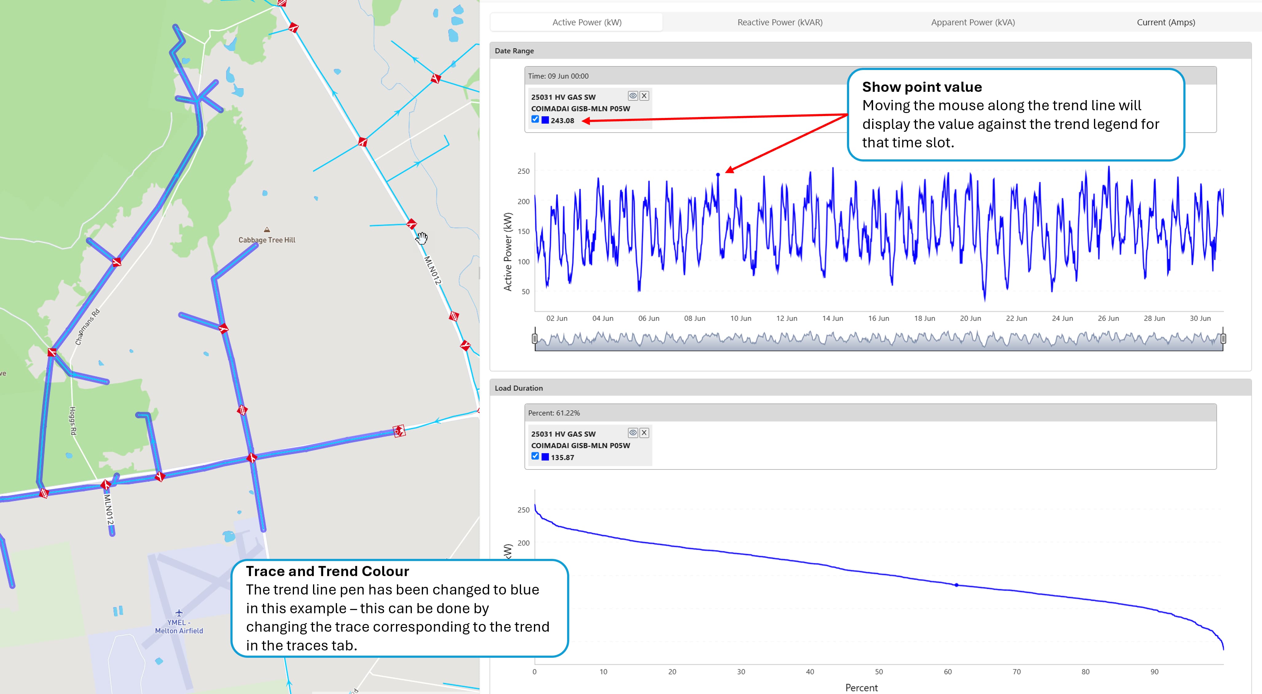
Immediately below the Date Range trend display is a load duration curve (LDC). An LDC is a graphical representation that plots the magnitude of electrical load (y-axis) against the duration (x-axis) for which it is equaled or exceeded, arranged in descending order from highest to lowest. It transforms chronological demand data into a format that highlights capacity requirements and usage. Unlike the date range trend, which shows the chronological order of load, the LDC does not show when a specific load occurs, only how long it lasts.
In many situations, you may notice a date range trend has periods of time where there is reverse power flow, that is, negative load. In these cases, the LDC still provides an indication of how much time the load is negative, and how much time at each negative value, however the percentage figure provided on the x-axis for negative load figures should be calculated as 100 minus the percentage value on the x-axis.
The screen shot below shows a typical load duration curve, immediately below the date range trend it was calculated from.
Comparing Trends
Both the Max/Min and date range trends allow more than one trend to be displayed on the same trend axis. This is achieved by selecting more than one trace from the "Selected Traces" dropdown. In the screen shot below, two date range trends are being compared for two separate reclosers.
Load Trend Performance and Min/Max Approximation
The underlying time-series load data used to generate trend displays is typically cached in server memory for distribution transformers. This enables high-performance trend retrieval for requests involving the HV network.
At the individual energy consumer level, however, caching all available load data in memory is often impractical due to the significantly larger data volumes involved. To maintain acceptable response times for trends that include individual energy consumer data, a number of client-side optimisations are applied.
For Min/Max trends, these optimisations can reduce the precision of the calculated results because the full underlying time series may not be evaluated. The UI therefore provides a configurable trade-off between performance and accuracy, allowing users to increase the amount of data considered when greater accuracy is required. This behaviour is described in the following section.
In the following discussions, the term "Supply Points" is used. A supply point is an object typically found in the GIS that has one or more customers connected to it. This is called an EnergyConsumer in the IEC CIM model. The individual customer associated with the Supply Point (or EnergyConsumer) is known as a UsagePoint in the IEC CIM model.
Min/Max Trend Approximations - How they work.
When a trend display includes individual Supply Points for which load data is not cached, the Min/Max trend is calculated using an approximation method.
The process is as follows:
- The system identifies the distribution transformers supplying the non-cached Supply Points included in the trend.
- For those distribution transformers, the system determines the highest-demand and lowest-demand days.
- The number of maximum-demand days and minimum-demand days selected is twice the Limit value configured for the Min/Max trend in the UI.
- The Min/Max trend for the individual energy consumers is then calculated using only load data from those selected days, rather than evaluating the complete available time series.
This approach reduces the amount of non-cached load data that must be retrieved and processed while targeting the days most likely to contain the minimum and maximum demand conditions.
When this approximation method is applied, an information message is displayed in the panel above the trends to indicate that one or more displayed trends have been calculated using approximated Min/Max values, as shown in the screenshot below.
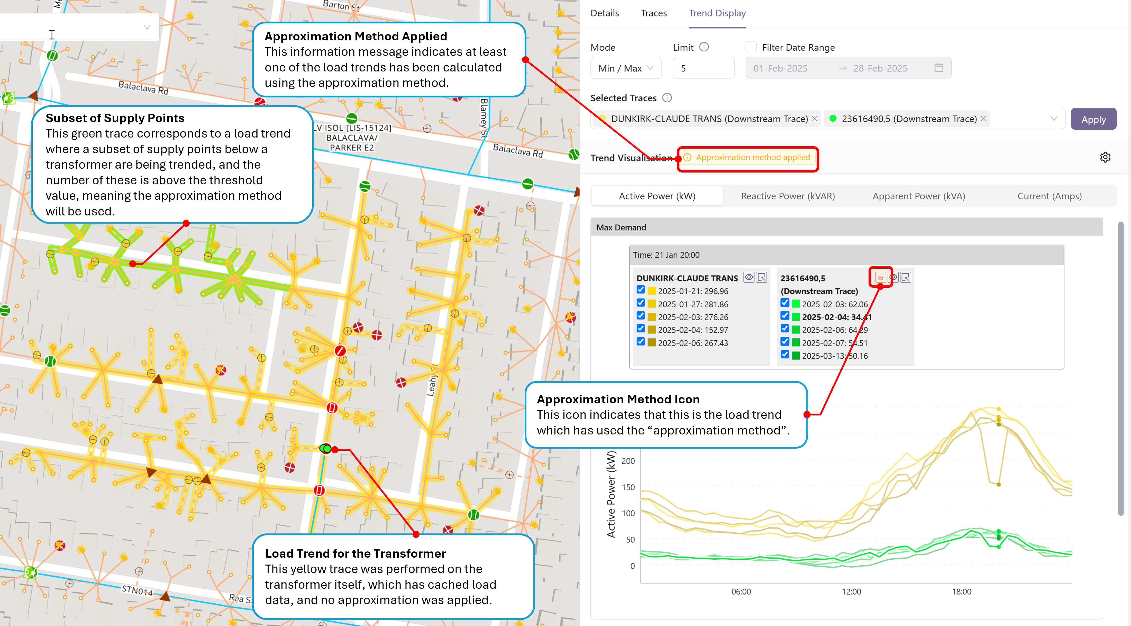
If you create a Min/Max load trend on a transformer, and then a load trend on the LV switch immediately below the transformer, the UI will indicate that an approximation method has been applied. However, in this case, because all the individual Supply Points have been included, the results will in fact be identical.
Improving the Precision
The accuracy of Min/Max trend results can decrease as the number of selected energy consumers becomes smaller, because the transformer-level maximum and minimum demand days are less likely to align exactly with those of the selected Supply Points.
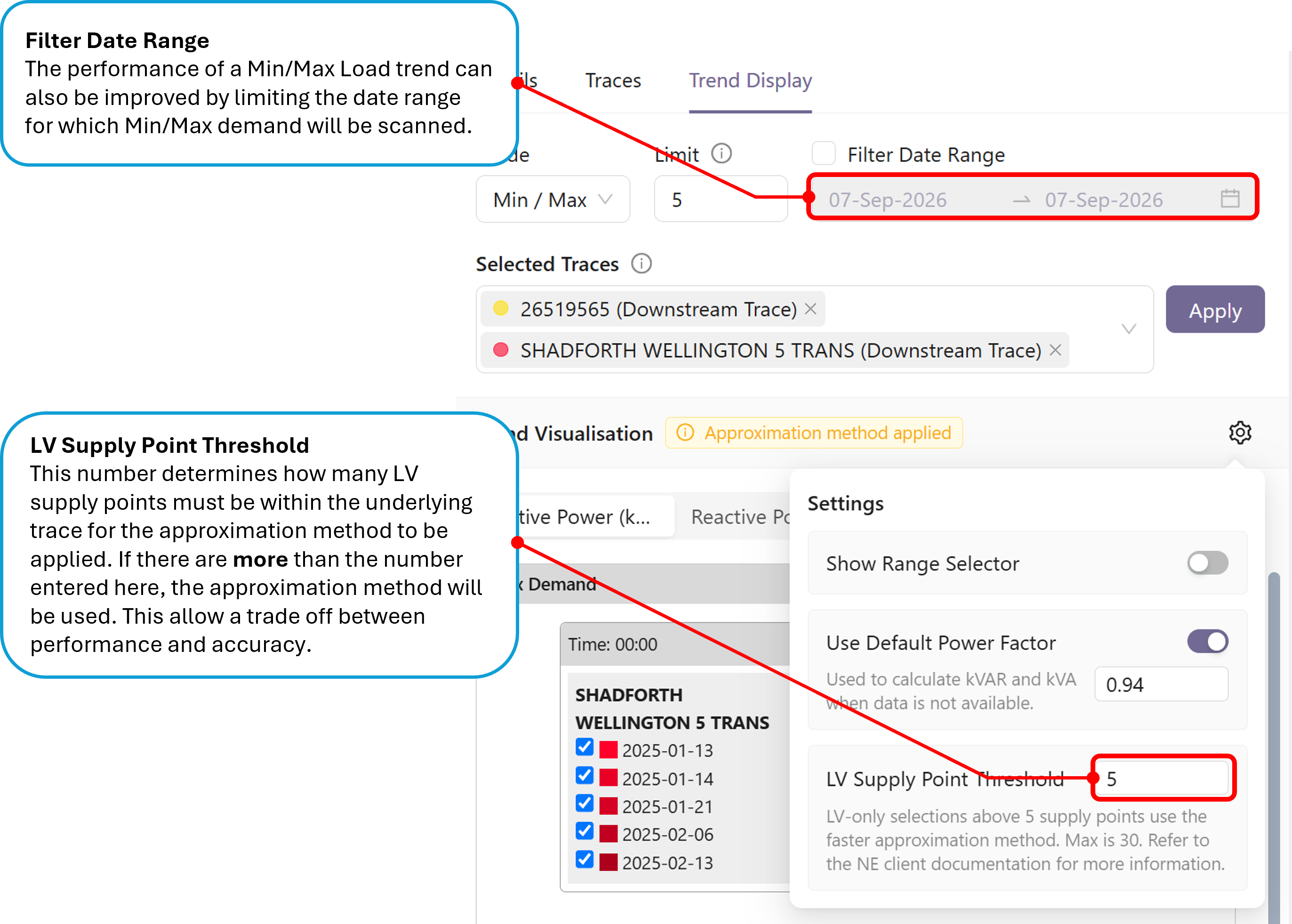
The UI provides an LV Supply Point threshold that controls when the approximation method is applied. As shown in the screenshot below, when the number of Supply Points included in a trend is below the configured threshold, the client does not use the approximation method. Instead, it requests a full scan of the available load data to determine the actual minimum and maximum demand periods.
Increasing the threshold improves the likelihood of obtaining exact Min/Max results for smaller selections of Supply Points, but at the cost of performance. The higher the threshold, the more frequently a full scan of the load database is required, which may increase trend calculation and response times.
There is an admin configurable upper value for the LV Supply Point Threshold - this is set at a value that provides the best outcomes for your organisations deployment. Please contact your system administrator if you believe this limit should be increased.
The performance of Min/Max load trends can also be improved by applying a Date Range Filter, to limit the number of days considered for the Min/Max trend.
Date Range Trend Limitations
For Date Range trends that include individual Supply Points with non-cached load data, the system applies a configurable limit to the maximum number of days that can be requested.
This limit prevents very large volumes of non-cached load data from being retrieved and processed in a single request, helping to maintain acceptable trend response times and overall system performance.
If the selected date range exceeds the configured limit, the Apply button is disabled and cannot be selected. Hovering the mouse over the disabled Apply button displays a message explaining that the requested date range exceeds the permitted limit.
To submit the trend request, reduce the selected date range until it falls within the configured maximum. Once the request is within the permitted range, the Apply button is enabled.
The limit applies only to trend requests that include individual non-cached Supply Point load data. Trends based entirely on cached load data are not subject to this restriction unless otherwise configured.