Studies
A study is a geographic visualisation of data displayed as an overlay on the map within Network Explorer. Studies are created using the Python SDK to create geoJSON features, which are then uploaded for display in the Network Explorer client via functions in the SDK. Naturally, this involves writing Python code to read and manipulate data to create the geoJSON visualisation.
Studies can also be created manually in the client, without using the Python SDK, to allow experimentation and debug. This is described below
Documentation on how to setup and use the Python SDK can be found here
The data used to create the study can come from any source, including the Energy Workbench itself. Examples of use cases for a study are:
- Displaying the results of a load flow simulation on the map
- Showing information about the network, such as length of lines, counts of objects, etc.
- Showing a heat map of solar penetration
- Showing the results of AMI analytics
Each study can contain multiple results: different collections of geoJSON that the user may switch between. For example, the first collection in the study may display per-unit voltage data from a load flow solution, while the second collection can provide a heatmap of the energy consumer density.
A tutorial on how to create and upload studies can be found in the python SDK examples documentation.
Creating studies requires an understanding of geoJSON and Mapbox style guides. The links below provide useful reference material.
Opening the Study
Once a study has been created, it can be opened from the Network Explorer client.
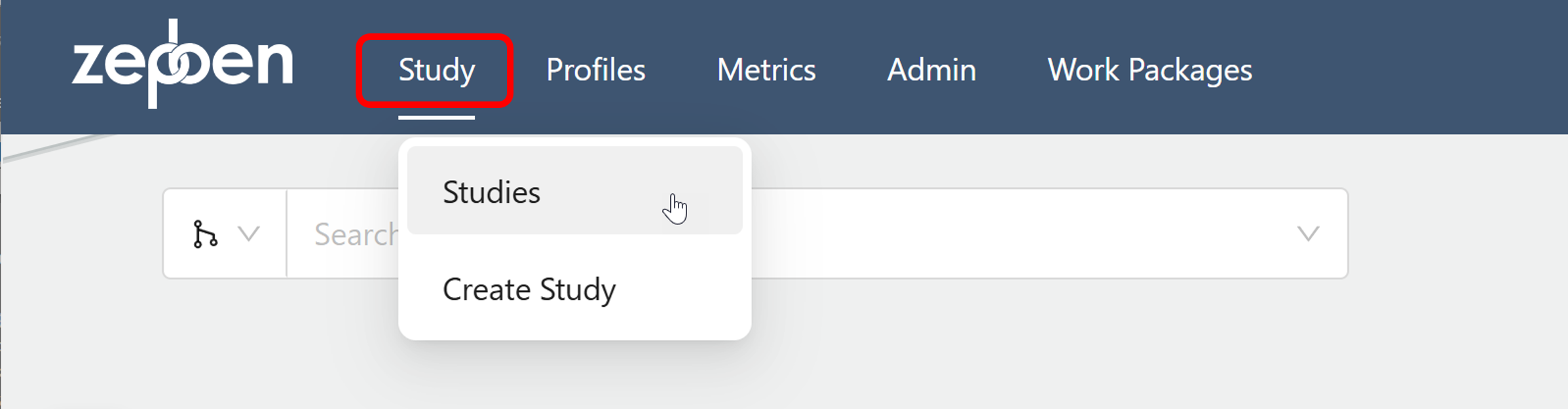
Clicking the "Studies" item will open a dialog box, as illustrated in the screen shot below. This shows all studies that have been created. Filters are provided on both the "Tags" and "Created By" columns to allow particular studies to be located.
The "Tags" column can contain multiple text entries, and is intended to be used to organise the studies sensibly.
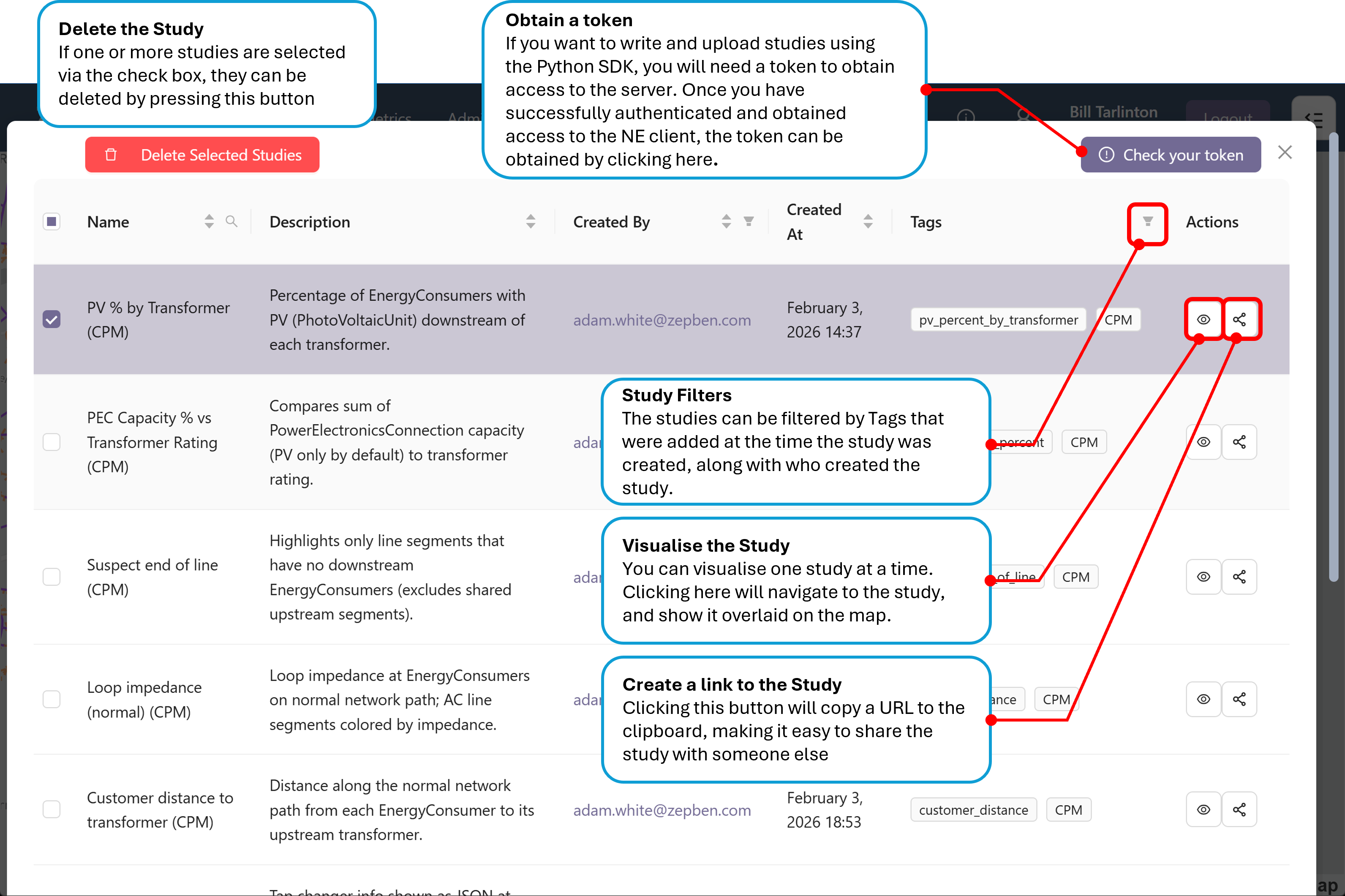
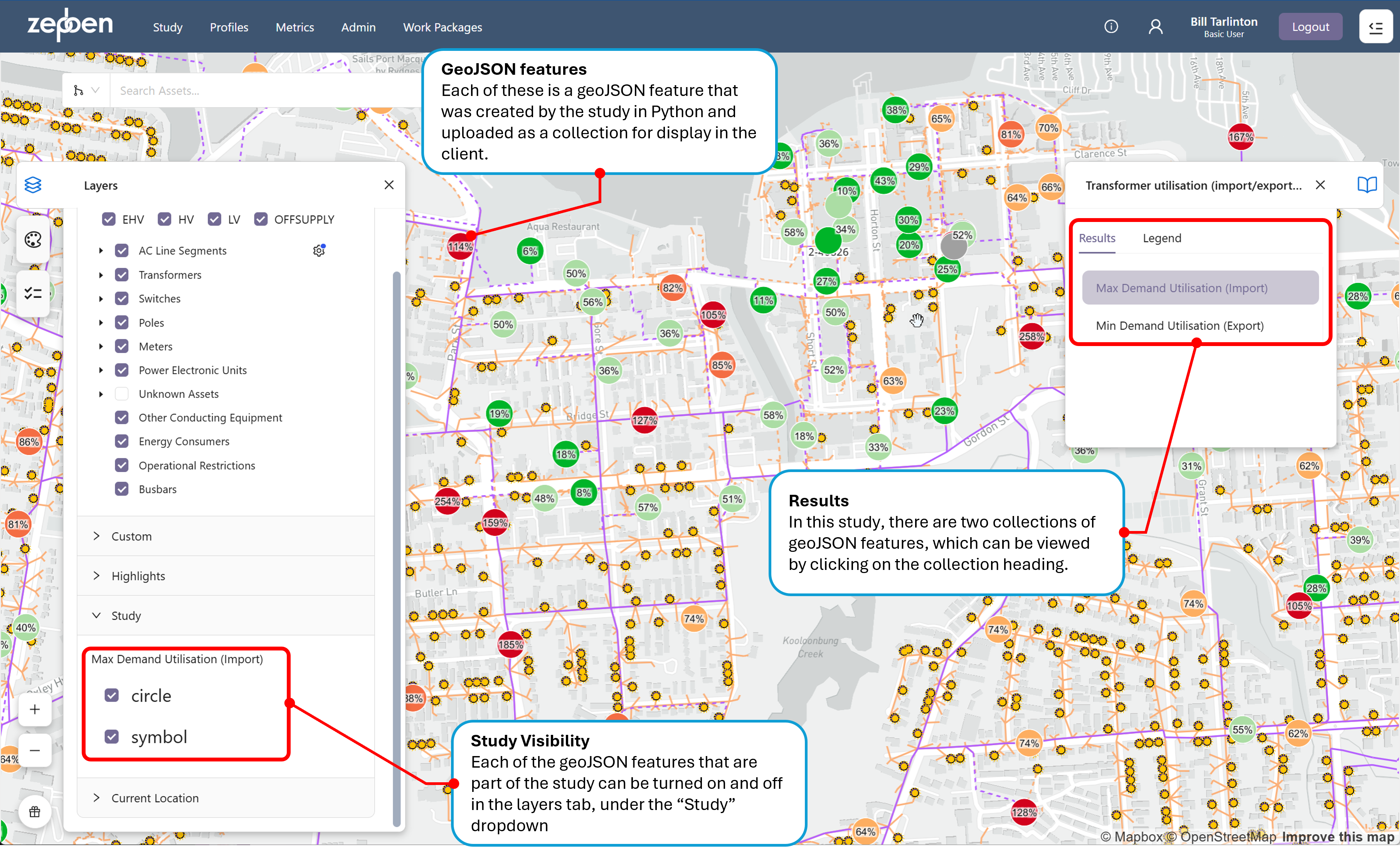
Clicking the view icon will display the study on the map, auto-zooming to the area of the network where the study has been overlaid. An example study is provided in the screen shot below.
In this study, an external data source that holds transformer utilisation has been combined with the spatial location of each transformer obtained from the Energy Workbench to create two geoJSON feature collections per transformer - one containing circles that have been colour coded to reflect the amount of transformer utilisation, and the other numbers showing the actual percentage utilisation.
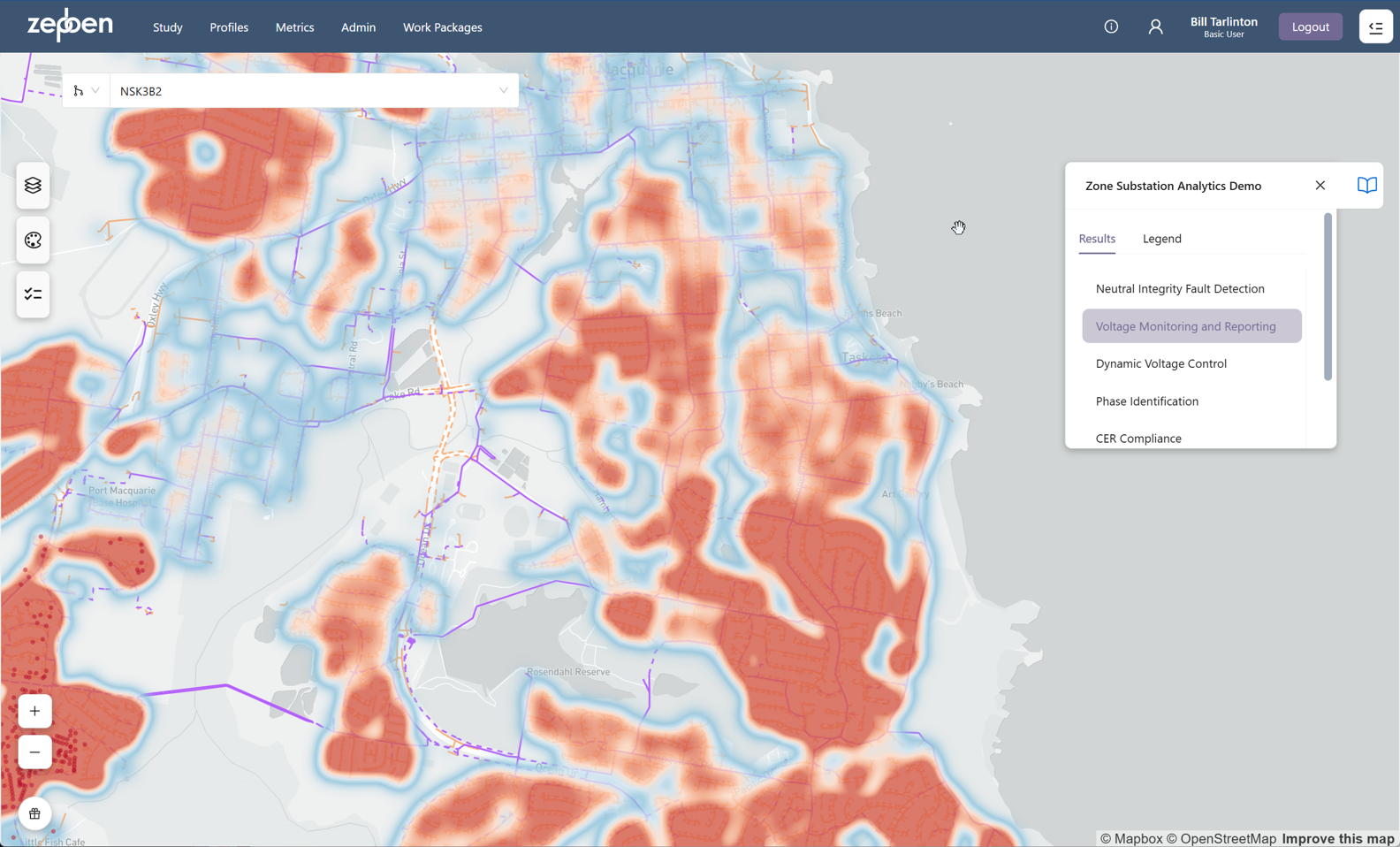
The screen shot below shows another example study, which has obtained data from an external AMI analytics system for voltage monitoring, CER compliance and other metrics, and generated various geoJSON collections to show the outcomes on a map. In the "Voltage Monitoring and Reporting" collection, a heat map has been used to show areas of the network that are at the higher and lower ends of the allowed voltage range.
Creating a Study Manually in the NE client
Studies can also be created directly in the client without needing the python SDK. This function allows you to create a single study that will be displayed on the map in the client by uploading a geoJSON and Mapbox layers file directly from your own machine. These studies are only visible to you and cannot be saved in the list of studies available from the python generated studies that appear in the studies list described earlier. Manually creating a study is done by selecting the "Create Study" option form the "Study" menu.
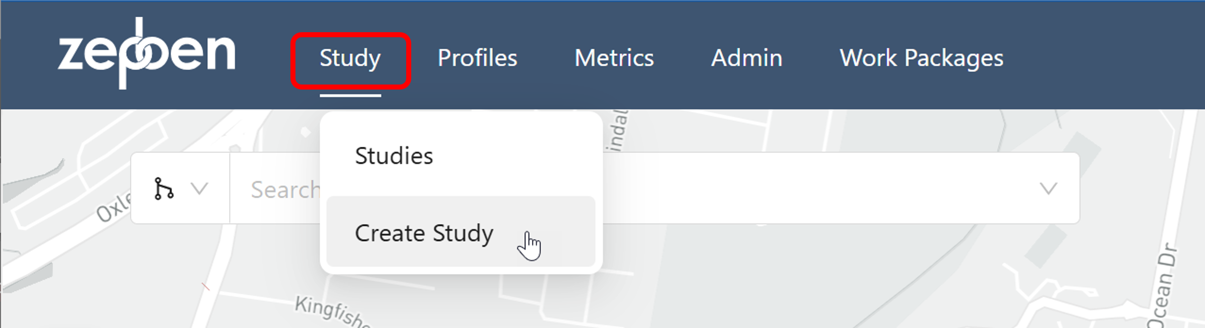
This will present the dialog box as illustrated in the screen shot below.
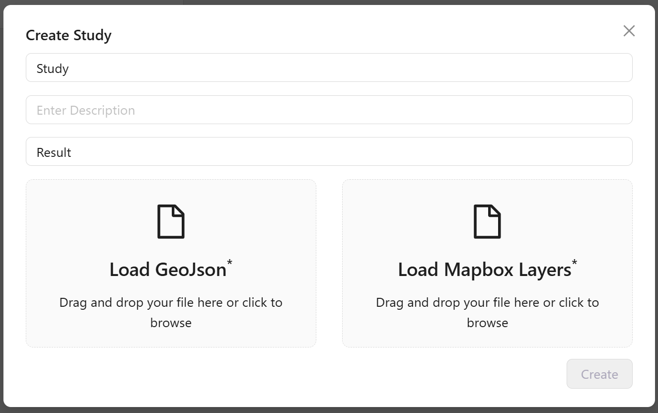
As shown on the screenshot, the geoJSON and Mapbox layers file can be uploaded by dragging the files onto the dialog box, or clicking to browse for the file on your local machine. The extension for the geoJSON file should be .geoJSON, and for the mapbox layers file, .json
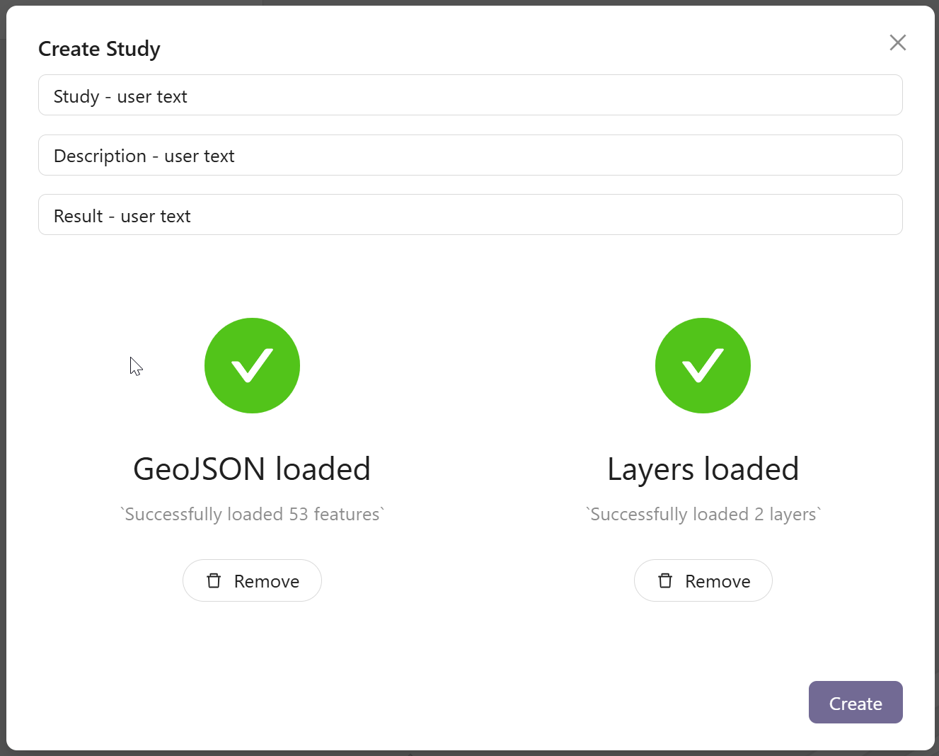
The three edit boxes at the top of the dialog box allow you to enter the study name, a description and a label for the results that displayed. Successfully uploading a geoJSON and Mapbox layer json fill will result in comforting green ticks in each box, and no error message, as illustrated below, where the three editable fields have also been updated.
This will present the dialog box as illustrated in the screen shot below.
Example geoJSON and mapbox layers
An example of a geoJSON feature collection and a corresponding set of mapbox layer definitions are provided below. If you cut and past these into files, they can be dropped into the "Create Study" dialog box.
Example geoJSON features
{
	"type": "FeatureCollection",
	"features": [
		{
			"type": "Feature",
			"id": "transformer6083",
			"geometry": {
				"type": "Point",
				"coordinates": [
					152.892322,
					-31.465109
				]
			},
			"properties": {
				"pv_percent": 50,
				"pv_percent_label": "50%",
				"pv_ec_count": 1,
				"ec_count": 2,
				"type": "pt"
			}
		},
		{
			"type": "Feature",
			"id": "substation_site208573",
			"geometry": {
				"type": "Point",
				"coordinates": [
					152.908476,
					-31.48886
				]
			},
			"properties": {
				"pv_percent": 77,
				"pv_percent_label": "77%",
				"pv_ec_count": 24,
				"ec_count": 31,
				"type": "pt"
			}
		},
		{
			"type": "Feature",
			"id": "substation_site202797",
			"geometry": {
				"type": "Point",
				"coordinates": [
					152.906038,
					-31.490112
				]
			},
			"properties": {
				"pv_percent": 13,
				"pv_percent_label": "13%",
				"pv_ec_count": 19,
				"ec_count": 144,
				"type": "pt"
			}
		},
		{
			"type": "Feature",
			"id": "substation_site210611",
			"geometry": {
				"type": "Point",
				"coordinates": [
					152.899482,
					-31.50194
				]
			},
			"properties": {
				"pv_percent": 0,
				"pv_percent_label": "0%",
				"pv_ec_count": 0,
				"ec_count": 2,
				"type": "pt"
			}
		},
		{
			"type": "Feature",
			"id": "transformer62089",
			"geometry": {
				"type": "Point",
				"coordinates": [
					152.903407,
					-31.490169
				]
			},
			"properties": {
				"pv_percent": 33,
				"pv_percent_label": "33%",
				"pv_ec_count": 1,
				"ec_count": 3,
				"type": "pt"
			}
		},
		{
			"type": "Feature",
			"id": "transformer10254",
			"geometry": {
				"type": "Point",
				"coordinates": [
					152.90951,
					-31.483019
				]
			},
			"properties": {
				"pv_percent": 71,
				"pv_percent_label": "71%",
				"pv_ec_count": 60,
				"ec_count": 84,
				"type": "pt"
			}
		},
		{
			"type": "Feature",
			"id": "substation_site202792",
			"geometry": {
				"type": "Point",
				"coordinates": [
					152.912923,
					-31.482338
				]
			},
			"properties": {
				"pv_percent": 0,
				"pv_percent_label": "0%",
				"pv_ec_count": 0,
				"ec_count": 2,
				"type": "pt"
			}
		},
		{
			"type": "Feature",
			"id": "transformer3386",
			"geometry": {
				"type": "Point",
				"coordinates": [
					152.916256,
					-31.478929
				]
			},
			"properties": {
				"pv_percent": 58,
				"pv_percent_label": "58%",
				"pv_ec_count": 57,
				"ec_count": 98,
				"type": "pt"
			}
		},
		{
			"type": "Feature",
			"id": "transformer5884",
			"geometry": {
				"type": "Point",
				"coordinates": [
					152.914762,
					-31.477135
				]
			},
			"properties": {
				"pv_percent": 17,
				"pv_percent_label": "17%",
				"pv_ec_count": 1,
				"ec_count": 6,
				"type": "pt"
			}
		},
		{
			"type": "Feature",
			"id": "transformer3407",
			"geometry": {
				"type": "Point",
				"coordinates": [
					152.914318,
					-31.478421
				]
			},
			"properties": {
				"pv_percent": 0,
				"pv_percent_label": "0%",
				"pv_ec_count": 0,
				"ec_count": 3,
				"type": "pt"
			}
		},
		{
			"type": "Feature",
			"id": "transformer63382",
			"geometry": {
				"type": "Point",
				"coordinates": [
					152.903924,
					-31.476421
				]
			},
			"properties": {
				"pv_percent": 58,
				"pv_percent_label": "58%",
				"pv_ec_count": 15,
				"ec_count": 26,
				"type": "pt"
			}
		},
		{
			"type": "Feature",
			"id": "transformer52497",
			"geometry": {
				"type": "Point",
				"coordinates": [
					152.901812,
					-31.479157
				]
			},
			"properties": {
				"pv_percent": 72,
				"pv_percent_label": "72%",
				"pv_ec_count": 34,
				"ec_count": 47,
				"type": "pt"
			}
		},
		{
			"type": "Feature",
			"id": "transformer6414",
			"geometry": {
				"type": "Point",
				"coordinates": [
					152.905256,
					-31.477183
				]
			},
			"properties": {
				"pv_percent": 85,
				"pv_percent_label": "85%",
				"pv_ec_count": 28,
				"ec_count": 33,
				"type": "pt"
			}
		},
		{
			"type": "Feature",
			"id": "transformer10017",
			"geometry": {
				"type": "Point",
				"coordinates": [
					152.906539,
					-31.476634
				]
			},
			"properties": {
				"pv_percent": 40,
				"pv_percent_label": "40%",
				"pv_ec_count": 4,
				"ec_count": 10,
				"type": "pt"
			}
		},
		{
			"type": "Feature",
			"id": "transformer59696",
			"geometry": {
				"type": "Point",
				"coordinates": [
					152.903726,
					-31.473304
				]
			},
			"properties": {
				"pv_percent": 77,
				"pv_percent_label": "77%",
				"pv_ec_count": 17,
				"ec_count": 22,
				"type": "pt"
			}
		},
		{
			"type": "Feature",
			"id": "transformer3662",
			"geometry": {
				"type": "Point",
				"coordinates": [
					152.906855,
					-31.47093
				]
			},
			"properties": {
				"pv_percent": 57,
				"pv_percent_label": "57%",
				"pv_ec_count": 42,
				"ec_count": 74,
				"type": "pt"
			}
		},
		{
			"type": "Feature",
			"id": "transformer3403",
			"geometry": {
				"type": "Point",
				"coordinates": [
					152.908513,
					-31.469345
				]
			},
			"properties": {
				"pv_percent": 60,
				"pv_percent_label": "60%",
				"pv_ec_count": 53,
				"ec_count": 89,
				"type": "pt"
			}
		},
		{
			"type": "Feature",
			"id": "transformer5247",
			"geometry": {
				"type": "Point",
				"coordinates": [
					152.896635,
					-31.471062
				]
			},
			"properties": {
				"pv_percent": 63,
				"pv_percent_label": "63%",
				"pv_ec_count": 36,
				"ec_count": 57,
				"type": "pt"
			}
		},
		{
			"type": "Feature",
			"id": "transformer55721",
			"geometry": {
				"type": "Point",
				"coordinates": [
					152.900842,
					-31.468412
				]
			},
			"properties": {
				"pv_percent": 56,
				"pv_percent_label": "56%",
				"pv_ec_count": 48,
				"ec_count": 86,
				"type": "pt"
			}
		},
		{
			"type": "Feature",
			"id": "transformer73674",
			"geometry": {
				"type": "Point",
				"coordinates": [
					152.897422,
					-31.460914
				]
			},
			"properties": {
				"pv_percent": 0,
				"pv_percent_label": "0%",
				"pv_ec_count": 0,
				"ec_count": 0,
				"type": "pt"
			}
		}
	],
	"styles": [
		"a78705fc-c437-4e74-a26e-ff07261b0f62",
		"7f5c064f-a6f2-4e19-8e7c-6c9375f00771"
	]
}
Corresponding Mapbox Layers
[
	{
		"id": "a78705fc-c437-4e74-a26e-ff07261b0f62",
		"name": "PV % by Transformer",
		"type": "circle",
		"minzoom": 12,
		"paint": {
			"circle-radius": 15,
			"circle-color": [
				"case",
				[
					"<",
					[
						"get",
						"ec_count"
					],
					3
				],
				"rgb(160,160,160)",
				[
					"step",
					[
						"get",
						"pv_percent"
					],
					"rgb(0,180,40)",
					10,
					"rgb(171,221,164)",
					25,
					"rgb(253,174,97)",
					40,
					"rgb(244,109,67)",
					60,
					"rgb(210,2,29)"
				]
			],
			"circle-stroke-color": "white",
			"circle-stroke-width": 1
		},
		"filter": [
			"==",
			[
				"get",
				"type"
			],
			"pt"
		]
	},
	{
		"id": "7f5c064f-a6f2-4e19-8e7c-6c9375f00771",
		"name": "PV Percentage",
		"type": "symbol",
		"minzoom": 12,
		"layout": {
			"text-field": [
				"get",
				"pv_percent_label"
			],
			"text-font": [
				"DIN Offc Pro Medium",
				"Arial Unicode MS Bold"
			],
			"text-size": 12
		},
		"paint": {
			"text-color": "white"
		},
		"filter": [
			"==",
			[
				"get",
				"type"
			],
			"pt"
		]
	}
]
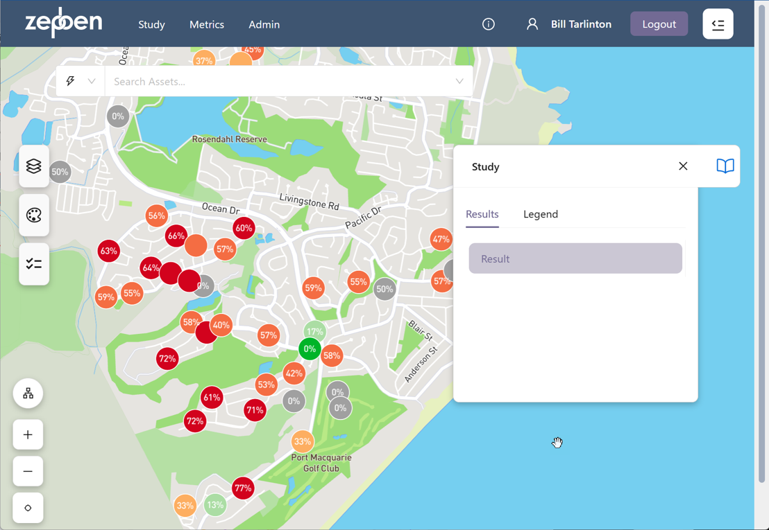
Doing this should render the geoJSON to appear in the map as illustrated in the screenshot below.
Limitations
The studies feature can render approximately 10,000 individual geoJSON features before the performance of the Network Explorer client begins to degrade. This will vary depending on the browser being used, and the CPU and the memory of the device running the application.